101 papers
$\newcommand{\Ef}[2]{\mathbb{E}_{#1}\left[#2\right]}$
Progress
Contents
- 1. Hierarchical Multi-Scale Attention for Semantic Segmentation (link)
- 2. Sequence Level Semantics Aggregation for Video Object Detection (link)
- 3. Taming Transformers for High-Resolution Image Synthesis (link)
- 4. Reformer: The Efficient Transformer (link)
- 5. Adaptive Computation Time for Recurrent Neural Networks (link)
- 6. A unifying mutual information view of metric learning: cross-entropy vs. pairwise losses (link)
- 7. pixelNeRF: Neural Radiance Fields from One or Few Images (link)
- 8. Object-Centric Neural Scene Rendering (link)
- 9. Universal Transformers (link)
- 10. Bottleneck Transformers for Visual Recognition (link)
- 11. Learning Deep Representations of Fine-grained Visual Descriptions (link)
- 12. Model-Agnostic Meta-Learning for Fast Adaptation of Deep Networks (link)
- 13. Joint Object Detection and Multi-Object Tracking with Graph Neural Networks (link)
- 14. Learning to Simulate Complex Physics with Graph Networks (link)
- 15. FetchSGD- Communication-Efficient Federated Learning with Sketching (link)
- 16. Learning Mesh-Based Simulation with Graph Networks (link)
- 17. GRAF: Generative Radiance Fields for 3D-Aware Image Synthesis(link)
- 18. mixup: Beyond Empirical Risk Minimization (link)
- 19. Deep Networks with Stochastic Depth (link)
- 20. An Image is Worth 16x16 Words: Transformers for Image Recognition at Scale (link)
- 21. How to train your ViT? Data, Augmentation, and Regularization in Vision Transformers (link)
- 22. Improving Text-to-Image Synthesis Using Contrastive Learning (link)
- 23. Momentum Contrast for Unsupervised Visual Representation Learning (link)
- 24. Improved Baselines with Momentum Contrastive Learning aka MoCov2 (link)
- 25. Emerging Properties in Self-Supervised Vision Transformers (link)
- 26. The Reversible Residual Network:Backpropagation Without Storing Activations (link)
- 27. MADE: Masked Autoencoder for Distribution Estimation (link)
- 28. Scaling Autoregressive Video Models (link
- 30. Multi-Task Learning Using Uncertainty to Weigh Losses for Scene Geometry and Semantics (link)
- 31. Universal Language Model Fine-tuning for Text Classification (link)
- 32. NeRF: Representing Scenes as Neural Radiance Fields for View Synthesis (link)
- 33. Character-level language modeling with deeper self-attention (link)
- 34. Transformer-XL: Attentive Language Models Beyond a Fixed-Length Context (link)
- 35. Stabilizing Transformers for Reinforcement Learning (link)
- 36. PointRend: Image Segmentation as Rendering (link)
- 37. Aggregated Residual Transformations for Deep Neural Networks aka ResNext (link)
- 38. Ab initio solution of the many-electron Schrödinger equation with deep neural networks (link)
- 39. GLIDE: Towards Photorealistic Image Generation and Editing with Text-Guided Diffusion Models (link)
- 40. Denoising Diffusion Probabilistic Models (link)
- 41. Improved Denoising Diffusion Probabilistic Models (link)
- 42. Denosing Diffusion Implicit Models (link)
- 43. GPT-4 Technical Report (link)
- 44. LLaMA: Open and Efficient Foundation Language Models (link)
- 45. Visual ChatGPT: Talking, Drawing and Editing with Visual Foundation Models (link)
- 46. Chain-of-Thought Prompting Elicits Reasoning in Large Language Models (link)
- 47. Mastering the Game of Go without Human Knowledge (link)
- 48. Thinking Fast and Slow with Deep Learning and Tree Search (link)
- 49. PromptChainer: Chaining Large Language Model Prompts through Visual Programming (link)
- 50. STaR: Self-Taught Reasoner Bootstrapping Reasoning With Reasoning (link)
- 51. Rosetta Neurons: Mining the Common Units in a Model Zoo (link)
1. Hierarchical Multi-Scale Attention for Semantic Segmentation (link)
Different image sizes work best for segmentation different types of objects in an image. Large regions benefit from small sizes enabling a model to get more context whilst fine details require high resolution. They propose a method to dynamiically combine the segmentations for different image scales in a cascaded hierarchical fashion with images decreasing in size. For each image scale a backbone segmentation network predicts a segmentation and an attention map. This attention is then “divided” between the segmentation for this image scale and the previous (larger) image scale and used to conbine segmentation outputs from the present and the previous layers to produce the final output for the present layer. This can be repeated an arbitrary number of times with the possibility of using different scales for training and inference (as they do). They achieve state of the art on Cityscapes for which they also use Cityscapes coarse annotations via auto-learning.
2. Sequence Level Semantics Aggregation for Video Object Detection (link)
Their method for video object detection works as follows: 1/ Given a frame and a region proposal in the frame, randomly sample $N$ other frames (which could from before or after this frame) 2/ Generate region proposals for these 3/ Get a similarity scores between the proposals in this frame and other frames 4/ For each proposal in this frame aggregate the proposals from other frames based on their similarity to this one (it is not clear how this is them combined with the proposal in the present frame) 5/ Make predictions as usual using the aggregated features (they use a Faster-RCNN type model) This way you are implicitly dealing with graph connecting objects between different frames in the video. The key idea is the semantic neighbourhood to which this gives rise is a source of more diverse features compared to the temporal neighbourhood where there is likely to be high feature redundancy. At test time they sample a larger number of frames and from those temporally later as well as earlier (if I understand right and which although it seems to benefit performance will limit application in live settings). They get SoTA on ImageNet VID and EPIC KITCHENS.
3. Taming Transformers for High-Resolution Image Synthesis (link)
Images are represented as a grid learning embeddings that is of a smaller size compared to the input. These grid then be flattened into sequence that is of a feasible size to train a large auto-regressive transformer model which can then be used to generate much large images than standalone transformers can. The embeddings are learned using a generative model (VQGAN). This model consists of an encoder which predicts a feature map. The feature vector of each pixel in the feature map is then matched to the nearest learned embedding and the resulting feature map of embeddings is input to a decoder which generates a image output. Having obtained this “codebook” of embeddings, a transformer model can be trained in an autoregressive manner to predict the next (according to some ordering of grid elements) embedding index as a $K$-way softmax output for $K$ embeddings. These are used to look up the embeddings from the codebook and input to the decoder to generate an image. The model outperforms a SoTA fully convolutional approach (PixelSNAIL) on a number of datasets as well as generating high quality high resolution images.
4. Reformer: The Efficient Transformer (link)
This is another approach to enable transformers to handle long sequences. The bottleneck is the attention map whose size is of order (N^2) where N is the sequence length. In this paper they note that the attention maps depend on the $\text{softmax}\left(\frac{QK^T}{\sqrt(d_k)}\right)$ they will dominated by elements which correspond to key and query vectors which are the closest to each other whilst other elements will be close to zero. Based on this insight they use a hashing mechanism which with high probability will place vectors that are close to each other (in the sense of having a large cosine similarity) in the same bins. The attention weights then only need to be found for pairs of keys and queries in the same bin with pairs in different bins giving rise to a weight of zero. If the the bin sizes are much smaller than $N$ then this approach will be a lot cheaper. One change they make to the regular model is to define the key vectors as the unit vectors in the direction of the query vectors so that $k_z = \frac{q_z}{\left \lVert q_z \right \rVert}$, which ensures that the hashes of $k_z$ and $q_z$ are the same and alleviates the problem of very uneven numbers of keys and queries in a bucket. I presumed that this means that 1/ they don’t do a key transform of the input in self-attention layers prior to applying attention; 2/ they don’t use the encoder outputs / memory to generate the key vectors when obtaining the attention weights to apply to the encoder outputs. I am not sure if this is the case but it looks like all the attention heads are self-attention with the difference that an element does not attend to itself unless there is no other element available e.g. if it is the first element in a sequence. They also experiment with adding reversible layers as in the reversible ResNet. The resulting model has a performance comparable to the regular transformer on a number of datasets and problems (enwiki8, WMT, imagenet64).
5. Adaptive Computation Time for Recurrent Neural Networks (link)
The key idea here is that a model should be able dynamically decide how much computation time to spend on a task based on its complexity. Consider an addition problem with a sequence of numbers of variable lengths. Adding a larger number will be more involved than adding a smaller one and the model should be able to adapt accordingly. This can also occur with non-sequential inputs where the prediction is more difficult to make for some inputs compared to others. The model works by modifying a normal RNN cell so that it kind of becomes an RNN itself. The difference is that the sequence involved is the number of computation steps rather than the data itself. We distinguish between data timesteps $t$ and number of compute steps $i$. Each iteration receives the entire input at timestep $t$ with an indicator when $i=0$ to inform the cell that the computation has just started for this data element. The cell generates and output and state at each compute step $i$ and the state is fed back for the next compute step. (When $i=0$ the state from the previous timestep, or when $t=0$ the initial state, is used). The cell makes an additonal prediction at every step $i$ which is used to decide if it should stop computing for element $t$. These predictions are also used to generate weights for aggregating the outputs and states from each compute step $i$. The model is trained using regular losses for the problem and an additional loss that penalises long computation times. The model outperforms baseline models which don’t use adaptive computation (i.e. where the RNN cell behaves like a regular RNN cell with just one compute step) on a number of algorithmic tasks (parity, logic, addition, sorting).
6. A unifying mutual information view of metric learning: cross-entropy vs. pairwise losses (link)
They show that simply training a ResNet50 classifier with cross-entropy loss will yield embeddings that can be used for image retrieval resulting in high recall (beating SoTA for 3 out of 4 datasets for which they run experiments). Various kinds of metric learning losses can be split into a “contrastive” and a “tightness” part. The first part encourages embeddings for similar images to lie close together and the second encourages those from dissimilar images to lie far apart. The goal is to maximise the mutual information $\mathcal{I}(\hat{Z}; Y)$ between the features and the labels. This can be expressed as $\mathcal{I}(\hat{Z};Y) = \mathcal{H}(\hat{Z}) - \mathcal{H}(\hat{Z} \vert Y)$. This will be maximised if features are far apart but those for a given class are close together. They show that the contrastive and tightness parts of other losses have similar properties to $\mathcal{H}(\hat{Z})$ and $\mathcal{H}(\hat{Z} \vert Y)$ respectively. The key difference between CE loss and these losses is that the later doesn’t incorporate any pairwise distances of the inputts. However they show that the CE loss can be represented as the sum of two components. The CE loss evaluated at the parameters $\theta^*_1$ and $\theta^*_2$ that minimise each component turns out to be a function of the pairwise distances of the inputs and this expression can be split into a contrastive and tightness part. This is defined as the Pairwise CE loss They argue that over the course of training $\theta^*_1$ and $\theta^*_2$ become very close so that $\theta^* \approx \theta^*_1 \approx \theta^*_2$ and thus the optimal CE loss at a given time-step is close to the Pairwise CE loss. Thus optimising the regular CE loss becomes an approximate upper-bound optimisation of the Pairwise CE loss.
7. pixelNeRF: Neural Radiance Fields from One or Few Images (link)
This is an extension of the NeRF architecture which leverages image features to enable training with limited numbers of views and to train a model that can represent different scenes. Instead of just asking the model “what is the colour at point $p$ of this scene when viewed from direction $d$?”, you now ask “what is the colour at point $p$ when viewed from direction $d$ of any scene relative to a view where point $p$ has features $z_p$?”. The way it works is by obtaining features for a known view and interpolating these features at the query point and passing them into the model as inputs along with the position and direction. A difference from the original model is that they also input the query viewing direction (which is relative to the viewing direction of the input image) since it is useful for the model to know how different this is relative to the input view. It is also possible to input more than one view at test time by independently obtaining features for each view and aggregating them before making a final prediction.
8. Object-Centric Neural Scene Rendering (link)
In the original NeRF model you just predict what is the colour along a direction $d$ to the camera origin. You only care about the outgoing rays from that point. You don’t think about the incoming light which is reflected from that point and gives rise to the colour in the image. In this paper they predict the fraction incoming light from different light sources that hits a point and use that to obtain the value of the outgoing ray. In contrast the original model simply predicts the final value of outgoing ray without considering how it comes about which prevents it from explicitly modelling interactions between objects. The train a separate model for each object and they compose the output using predictions from different models. Their model can also be used to predict shadows due to the some other object obstructing the light as well as secondary light rays that result from primary rays getting reflected from an object (and indeed the model can accomodate an arbitrary number of bounces).
9. Universal Transformers (link)
The model in this paper is inspired by the Adaptive Computation Time (ACT) RNN but applies this approach to a Transformer. Similar to the regular Transformer model they use an encoder-decoder architecture where the encoder block comprises a self-attention block and a transition block (plus LayerNorm and Dropout) and the decoder block comprises self-attention, memory attention and a transition block. The key difference is that they have just a single encoder and decoder block. Encoding consists of applying the same encoder block, initially to the input and then to the output from the previous application for a number of timesteps. The output of this is passed to the decoder which is then repeatedly run for a number of timesteps. The number of timesteps can be determined beforehand or decided dynamically on a per-symbol basis similar to ACT-RNN using a halting mechanism as in ACT-RNN to decide whether to stop computing for a particular symbol. The difference is that since the whole sequence needs to be present each time to use in self-attention, the output for the symbols which have been halted is simplied copied over to the next stage. This model is particularly good at algorithmic tasks at which the regular transform struggles. They show that unlike the regular Transformer it is Turing-complete. It also outperforms regular transformers on language tasks and manages to get SoTA on the LAMBDADA language modelling task.
10. Bottleneck Transformers for Visual Recognition (link)
This paper adopts a simple but effective approach of replacing lower resolution blocks of ResNet with Attention blocks and achieves instance segmentation performance which surpasses the previous best published results using a single model and single scale.
ResNet has residual blocks of the form {Conv1x1(N1, N2)->Conv3x3(N2, N2)->Conv1x1(N2, N3)} where N1 > N2, N2 < N3 (except for the first conv N2 = N1). Compare this to the regular transformer which has the form {Embedding(T, D1)}->[{Attention(D1, D1)}->{Dense(D1, D2)->Dense(D2, D1)}]+ where curly brackets {..} indicate residual blocks and D2 > D1 and the number of tokens T may also be larger than D1. If you unroll it a bit you get {Embedding(T, D1)}->{Attention(D1, D1)}->{Dense(D1, D2)->Dense(D2, D1)}-{Attention(D1, D1)}->{Dense(D1, D2)->Dense(D2, D1)}.... Now if you move the skip connection so that it begins and ends between the Dense blocks (or before the Embedding block the first time) you get {Embedding(T, D1)->{Attention(D1, D1)->Dense(D1, D2)}->{Dense(D2, D1)-Attention(D1, D1)->Dense(D1, D2)}->{Dense(D2, D1)->...}->..., which makes the residual blocks into bottleneck blocks. The one difference when using this type of block in ResNet is that the dense layers are replaced with convolutional layers.
They use relative positional encodings (which were found to be better than absolute ones). While models like ViT replace CNNs with Transformers, this is a hybrid backbone. Differently from DETR, this uses Transformer modules in the feature extraction step and uses regular detection heads whereas DETR uses a ResNet backbone followed by a Transformer based detection module. The resulting model named BoTNet also improves over various baseline architectures (SENets, Efficients, ResNets of different sizes) on ImageNet.
11. Learning Deep Representations of Fine-grained Visual Descriptions (link)
The task is to learn features from text descriptions of images of different classes that can be used for image retrieval and zero-shot classification. The way zero-shot classification works in this case is that you have text features from different classes and you pick the class whose average embedding yields the highest dot product with a given image. These will be new classes not seen at training time. The idea is that the model learns to project text containing information about a class to the same feature space as an image from that class.
The data consists of the Caltech Birds dataset and Oxford Flowers dataset both of which have 100 or more classes and they obtain their own fine grained text annotations
Given an image embedding $\theta(v)$, find the class $y$ such such that the average dot product of the text embeddings from that class $\phi(t)$ with $\theta(v)$ is maximised.
\[F(v, t) = \theta(v)^T\phi(t) \\ f_v(v) = \underset{y \in \mathcal{Y}}{\arg \max}\mathbb{E}_{t \sim \mathcal{T}(y)}\left[F(v, t)\right]\]This is also reversed to classify the text embedding (although this is only done during training).
The image embeddings are fixed but the model is described as symmetrical in the sense that there is a pair of losses.
\[\frac{1}{N} \sum_{n=1}^N l_v(v_n, t_n, y_n) + l_t(v_n, t_n, y_n)\]One encourages all text embeddings from a given class to lie close to an image embedding from that class and the other encourages each text embedding from a class to lie close to all the images from that class. They experiment with various encoders to obtain the text features and find that a Word-CNN-RNN trained on fine-grained annotations and the symmetrical loss is successful in most cases but for Caltech Birds, just using one-hot encoded attributes as the input does better for retrieval.
The loss $l_v$ is as follows and $l_t$ is similar with $v$ taking th place of $t$, where is $\Delta(y_n ,y)$ is the 0-1 loss:
\[l_v(v_n, t_n, y_n) = \max(0, \delta(y_n ,y) + \mathbb{E}_{t \sim \mathcal{T}(y)} \left[F(v_n, t) - F(v_n, t_n)\right])\]This is the average difference between $F(v_n, t), t \sim T(y)$ and $F(v_n, t_n)$ maximised over all classes $y$.
- Other $t$ from same class have higher dot products -> minimise loss
- Other $t$ from different class have higher DP -> minimise loss
- Other $t$ from same class have lower dot products -> do nothing since the difference term will be negative as the 0-1 loss $\Delta(y_n ,y)$ is 0 so the loss is 0. this makes sense because though if the average difference for $y_n$ negative but also the largest average difference across all classes, it follows that all other classes have a negative average difference which is moreoever larger and embeddings these classes must be therefore have less similar dot products on average. So actually is $y_n$ whose embeddings have the most similar dot products with $v$ compared to $t_n$.
- Other $t$ from different class have lower DP -> minimise loss until the average difference is 1 (the negative of the 0-1 loss which is 1).
12. Model-Agnostic Meta-Learning for Fast Adaptation of Deep Networks (link)
For a set of tasks $\mathcal{T}_i$ you find the loss gradient and update separate parameters for each of the $K$ examples of the task using the ‘train-train’ data. The parameters of the model are now the ‘adapted’ parameters $\theta_i$. Then you find the average loss for each task using its adapted parameters and the ‘train-test’ data and find the gradients of these with respect to the shared parameters. So basically you do what is like a training step for each task, testing the resulting models using task specific parameters and finally learning shared parameters. To evaluate you fine-tune for 1 or more steps on ‘test-train’ examples and find the metrics on the ‘test-test’ examples. At the time it was published it beat state of the art on few-shot learning tasks for Omniglot and ImageNet.
13. Joint Object Detection and Multi-Object Tracking with Graph Neural Networks (link)
The model jointly learns to detect and track objects by linking features between frames using a Graph Neural Network. Feature maps are generated for pair of consecutive frames (time steps $t-1$ and $t$). CenterNet is used to detect objects in the frame at timestep $t$.
To associate objects between frames, an identity embedding is generated for each object. RoIAlign is used to crop features for the detections that have already been made in the previous frame. Each pixel in frame $t$ is considered as a potential object’s centre location and a graph is construct between the objects in the previous frame and all the pixels features within a neighbourhood in frame $t$. This is empirically justified since objects don’t move too much across frames and avoids having to consider all possible pairs which would be computationally expensive.
Features in each layer of the graph network are updated using GraphConv as follows:
- Generate features for each node via a layer $\rho_1$
- Generate features for each of its neighbours via $\rho_2$
-
Sum all of these to get the output feature:
\[h_l^i = \rho_i\left(h_{l-1}^i\right) + \sum_{j \in \mathcal{N}(i)}\rho_2\left(h_{l-1}^j\right)\]
Although nodes in framee $t$ are not directly connected to each other if the graph network has more that one layer information can propagate between detections in the same frame through tracklets.
The model can thus be jointly trained to detect and to associate detections with “tracklets” from earlier frames. At inference time I think you start by detecting objects in the first frame and then using those as tracklets for the subsequent frame. Objects are paired with previous objects by calculating a similarities between the identity embeddings of the detections in the present and tracklets from previous frames. The Hungarian algorithm is then used to determine the best assignment of detections to tracklets. They also continute to retain tracklets for a few frames even if they are not matched to any object in the subsequent frame and similarly unmatched detections above a confidence level are kept.
They improve on the SoTA on a number of metrics on the MOTChallenges.
14. Learning to Simulate Complex Physics with Graph Networks (link)
In this paper they train a model to generate physics simulations. They input the states of several particles (e.g. those that comprise simulated fluid) at a given time, where a state includes position, velocities from earlier timesteps, static material properties and global system properties like forces and global material properties. A simulation consists of a trajectory of consecutive states. The goal is then to predict the acceleration at the next timestep from which the velocity and position can be estimated using semi-implicit Euler integration which updates velocity using the previouss velocity and the predicted acceleration and position using the newly estimated velocity and the previous position. In this way the predicted acceleration can directly influence the position estimate.
A graph network is used in which each particle is assigned to a node with edges added between nodes that correspond to particles with a radius $R$. They try two approaches, one where the absolute values of the particles are used in which case edges don’t have any features, and another where the relative positions are used in which edge features are based on the distance and displacement between the particles. A processor then runs $M$ steps of learned message passing updating the graph each time and returning a final graph. A decoder is then used to obtain the dynamics information from each note of the final graph.
At training time random pairs of consecutive timesteps are sampled from the training trajectories and the future state (here just the position) is predicted. At inference time this step is repeated to predict an entire trajectory. During inference the model’s own noisy predictions are used to generate subsequent predictions. Because of this they also add noise to input positions during training to make the model more robust to noisy inputs.
They manage to generate realistic looking simulations for a variety of materials and environments.
15. FetchSGD- Communication-Efficient Federated Learning with Sketching (link)
In this paper they propose a new method of computing gradient updates in federated learning. The gradients are computed locally on the client as usual but they are compressed using a data structure called Count-Sketch $\mathcal{S}$. It turns out that $\mathcal{S}$ is linear so that $\mathcal{S}(x + y) = \mathcal{S}(x) + \mathcal{S}(x)$ which means that the summed values after Count-Sketch has been applied to gradients is equivalent to applying it after summing all the gradients. Here they say that $\text{topk}\mathcal{S}(g)$ is roughly the same as $\text{topk}\mathcal(g)$.
An issue with FedAvg the classic approach is that it requires download and upload of the entire model each time. Moreover unlike other compression schemes FetchSGD only involves one communication round with any client. It also does not need to store state locally nor does it need to update all the weights each time.
Experiments on different tasks and datasets show that it performs better at higher compression levels compared to other algorithms.
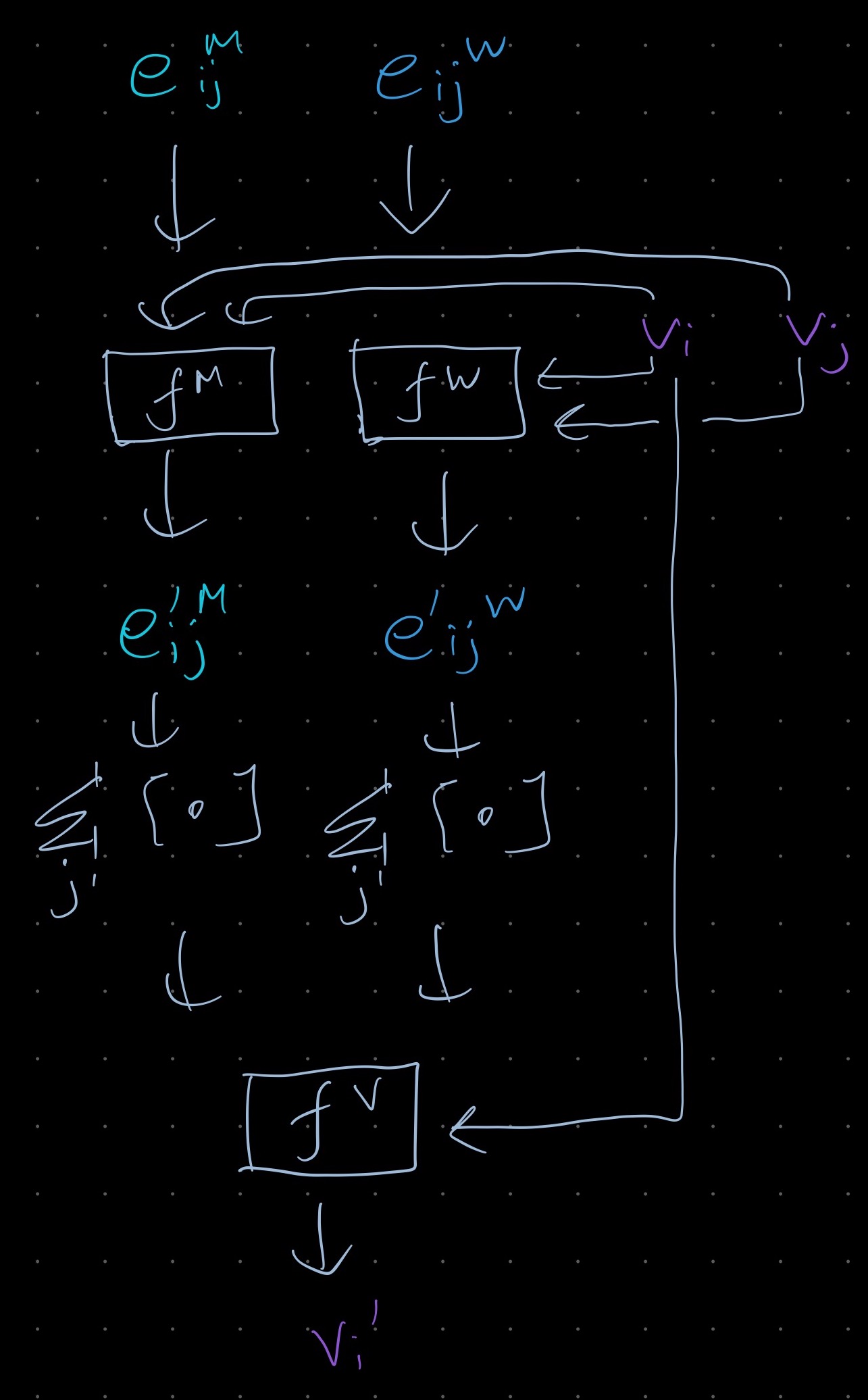
16. Learning Mesh-Based Simulation with Graph Networks (link)
At each timestep there is a mesh $M_t = G(V, E^M)$. Each node $i$ has a mesh space co-ordinate $\mathbf{u}_i$ and additional dynamical quantities $\mathbf{q}_i$ which are the ones that getting estimated. You can have Eulerian and Lagrangian systems, where the later have an additional coordinate $\mathbf{x}_i$ which describes the dynamical state of the mesh in 3D space.
The graph is a direct mapping from the mesh but in Lagrangan systems it has additional world space edges. In simple terms this seems to mean edges between nodes that are not directly “connected” in a material sense but come close to each other for example positions on opposites sides of a piece of cloth that come near to each other when the cloth is folded but far from each other when connected along the cloth. Other examples include points on two different meshes such as points on a ball that hits the cloth.
These edges are assigned to pairs of nodes that are within a radius $r_W$ which is on the order of the smallest edge lengths in the mesh and which are not connected by the mesh edges. (Question: what exactly is “non-local”?)
The input features at the mesh edges $e_{ij}$ are the relative displacement between the positions of their corresponding nodes $\mathbf{u}_i - \mathbf{u}_j$ and the norm of this $\lvert \mathbf{u}_{ij} \rvert$. Not using relative encoding for edges leads to worse performance.
In addition both the mesh and world edges get the world-space displacement vector $\mathbf{x}_{ij}$ and its norm. (I am not quite sure what this vector \mathbf{x}_{ij} actually is). All the dynamical quantities $\mathbf{q}_i$ are assigned as node features along with a one-hot node type feature. The input features for the nodes, the mesh and the world edges are all transformed to latent encodings via an MLP.
The processor consists of $L$ blocks, where the blocks are as illustrated below. It looks like you concatenate the input features and then uses an MLP with a residual connection to update the edges and nodes. I think that message passing comes about since you are first updating the edges and then using those to update the nodes. More message passing steps improve MSE but are costly.
The decoder then predicts various properities $\mathbf{p}_i$ for each node using the node features after the final processor block. The properities are interpreted as higher order derivatives of the node position and the position is estimated via Euler forward integration. Additional properties such as pressure or stress are also predicted. When second order values (e.g. acceleration) are predicted earlier velocity values are also input but using too much history leads to overfitting.
Remeshing involves changing the mesh after determining which regions of the mesh require higher resolution. A sizing field tensor based on heuristics that depend on the domain is typically used whereby the edge vector $u_ij$ is transformed by a sizing field tensor $S(u)$ and if the dot product of $u_{ij}$ with this is greater than 1 then edge is considered too long and is split up using a remeshing algorithm that is not domain dependent. They instead try to learn the remeshing tensor by using a similar model as described above by predicted a sizing field tensor for each node.
The model is supervised on the L2 loss between the nodes predictions and the ground truth. It is only trained to predict the next step but at inference time it is rolled out for longer trajectories. Using noisy data at training time makes it more robust to variations encountered when rolling out for longer steps.
It generates visually similar predictions for simulations of moving fabric, airfoils, compressible and incompressible fluids. They also identify a number of key features and advantages relative to other models:
-
It is faster than the solvers used to generate the ground truth data.
-
You can run generate long trajectories even though it is only trained to predict valus at the next step
-
It appears to be independent of resolution and scale allowing you to train on smaller meshes but run inference on larger ones. This might be because it learns the underlying physical processes.
-
Grid based models need more cells to represent the same simulation but despite that seem to underperform at small scales.
-
The improved performance over a particle based method GNS suggests that use of a mesh and message passing seems to be important. However using world-space edges is also appears to be important.
17. GRAF: Generative Radiance Fields for 3D-Aware Image Synthesis(link)
- Sample the follows
- Parameters of a translation and a rotation matrix from a distribution $p_\epsilon$. They use a uniform distribution over the upper hemisphere with the camera facing towards the origin and in some cases vary the distance from the origin to the camera.
- A centre location and what they describe as “scale” but seems to be a stride from the image. The centre x-y coordinates are uniformly sampled from across the image domain and the scale is sampled from a continuous uniform distribution between $1$ and $S$. Values are sampled from this continuous space over the image using interpolation.
- Latent vectors $\mathbf{z}_s$ and $\mathbf{z}_a$ for object shape and appearance, from a standard normal distribution.
- Based on the patch location, the transformation matrices and the camera intrinsics the 3D camera rays corresponding to any point in the patch can be determined. To predict the colour and volume density at a point $p_i$ in the patch do the following:
- Sample $N$ 3D points $\mathbf{x}_i$ along the ray $\mathbf{d}_i$ that corresponds to $p_i$.
- Encode these points using a positional encoding: $\gamma(\mathbf{x_i})$
- Concatenate with the shape latent $\mathbf{z}_s$ and input to an MLP to predict an encoding $\mathbf{h}$
- Using $\mathbf{h}$ by itself to predict the volume density $\sigma$
- Encode the direction: $\gamma(\mathbf{d_i})$
- Concatenate with $\mathbf{h}$ and the appearance latent $\mathbf{z}_a$ to predict the colour $\mathbf{c}$
- So far the key differences from NeRF are that you have a couple of additional stochastic inputs and you also restrict the input points to lie within an patch as opposed to anywhere within the locations the comprise the training set. A further difference from NeRF is how the predictions are supervised. Instead of using ground truth colour and volume density as targets, they train discriminator which receives as input a real image patch from the same patch sampling distribution and predicts whether it is real or fake. It would appear that this patch can come from any valid location in a ground truth image and can have a different stride compared to the input patch.
- Key features and results:
- The model gets a better (lower) FID on various datasets compared to the voxel based GAN approaches PlatonicGAN and HoloGAN.
- It also does well at higher resolutions including when not trained with images at those resolutions compared to these models, which are also prevented due to by their voxel based representation from generating very high resolutions.
- Qualitatively it can be seen that the model is good at disentangled different attributes like pose, shape and appearance - changing the pose seems to result in images in which the same object seems to be present only oriented differently whereas the other models also change the appearance of the object and / or have artifacts.
- Moreover varying the appearance and shape latents one at a time results in images where the only the appearance or the shape change.
- A lower 3D reconstruction loss is further suggestive of multiview consistency.
18. mixup: Beyond Empirical Risk Minimization (link)
Basic summary
Data augmentation that uses linear inductive bias to input values interpolated between pairs of samples and labels in different classes, which acts as a vicinity distribution that approximates the problem of maximising the log likelihood instead of using ERM. The motivation behind how it works is that linearity is a good inductive bias for Occam’s razor. The mixup probability is sampled from $\beta{\alpha, \alpha}$ where $\alpha$ is a hyperparameter. For mixed-up samples a correct prediction for the purposes of accuracy is either of the interpolated classes. Mixup improves baselines (or at least does no worse in a few cases) for CIFAR-10 and 100, ImageNet, Google commands (speech), Tabular data from UCI and also improves robustness to noisy data and adversarial examples.
More on ERM
-
You want to minimise the risk of a hypothesis $f$ which is the expected value of the error between $f(x)$, the prediction, and $y$ the true label where the expectation is with respect to the true data distribution $P(x, y)$ \(R(f) = \int{L\left(f(x), y\right)dP(x, y)}\)
-
Since you don’t know the true data distribution you approximate it via a uniform distribution over the training data $x^{(i)}, y^{(i)}$, consisting of $N$ samples:
\[\hat{P}(x, y) = \frac{1}{N}\sum{i=1}^{N}\delta(x=x^{(i)})\delta(y=y^{(i)})\] -
This yields the following empirical risk over the training set:
\[\hat{R}(f) = \frac{1}{N}\sum_{i=1}^{N} L(f(x^{(i)}), y^{(i)})\] - However we can also use some other approximation to the true distribution for example “Vicinal Risk Minimisation” where we consider the probability of a virtual pair $\tilde{x}, \tilde{y}$ given the training data $x^{(i)}, y^{(i)}$.
-
The one that they propose is as follows:
\(\lambda \sim B(\alpha, \alpha)\) \(\tilde{x}^{(i, j)} = \lambda x^{(i)} + (1- \lambda) x^{(j)}\) \(\tilde{y}^{(i, j)} = \lambda y^{(i)} + (1- \lambda) y^{(j)}\) \(\hat{P}(\tilde{x}, \tilde{y} \vert x^{(a)}, y^{(a)}) = \frac{1}{N}\sum_{b=1}^{N}\mathbb{E}_{\lambda}\left[\delta(\tilde{x}=\tilde{x}^{(a, b)})\delta(\tilde{y}=\tilde{y}^{(a, b)})\right]\)
Results in more detail
- Bigger models and those trained for longer tend to benefit more from mixup (noted for ImageNet, Google commands)
- Large values of $\alpha$ do worse than smaller ones for classification tasks (noted for ImageNet)
- Mixup converges at the same rate as ERM (noted for CIFAR-10) to best test error
- Mixup with dropout tends to do the best for noisy data
- For speech mixup is applied to spectrogram but could also be applied to waveform
19. Deep Networks with Stochastic Depth (link)
ResNet models are trained with stochastic depth by deciding according to some probability for each skip connection where or not to use only the identity part thereby dropping this layer. A simple approach is to linearly decrease the probability of keeping the layer based on a hyperparameter $p_{L}$ which is the probability for the final or $L-th$ layer which is used during training whilst during test the layer is scaled by the probability of keeping the layer. This leads to faster training time since the expected number of active layers at each step is lower than the length of the network (~75% using the linear approach) and they suggest that it could alleviate the vanishing gradient problem and diminishing feature reuse (like vanishing gradients but for forward pass whereby features are washed out by repeated multiplication or convolution with randomly initialised weights) by allowing shorter paths to the output from each layer as well as [something else]. They also suggest that this works like an ensemble of networks of different depth where at test time each layer is weighted by the probability that it will be present in a given model. The model does significantly better regular ResNets on CIFAR-10 (which it sustains with a 1000+ layer model whose original configuration fails to do better than a 110 layer model but this model does better than the 110 layer one as well), CIFAR-100, has a slight advantage for SVHN but does not improve on ImageNet.
20. An Image is Worth 16x16 Words: Transformers for Image Recognition at Scale (link)
The model proposed in this paper is a straightforward extension of a regular transformer where you divide the image into non-overlapping patches of a given size e.g. $16 \times 16$, flatten each of these and transform them into a sequence of input embeddings which are concatenated to a CLS token at the start of the sequence. Besides that it looks like a regular transformer encoder with a few minor architectural changes (e.g. gelu instead of relu, more dropout layers when dropout is used) and the output corresponding to the CLS token is input to a final classifier head. Importantly there is no inductive bias since the positional encoding is 1D and only during fine-tuning where larger images are used and the encodings interpolated in 2D is any inductive bias introduced. ViT pre-trained on JFT-300M does as well as or better than other models thus pre-trained when fine-tuned on a number of different datasets. Some points about scaling:
- For smaller datasets the inductive bias of conv nets seems to confer an advantage relative to ViT models of similar size but this disappears for larger datasets.
- For models of comparable accuracy, ViT tends to be faster than ResNet (alternatively for models of comparable speed, ViT tends to be more accurate) although for smaller models hybrids tend to do better than ViTs
- Performance does not saturate with model size for the sizes tried
- You need to pre-train on a larger dataset to benefit from using a larger model (e.g. JFT300M v ImageNet for ImageNet).
21. How to train your ViT? Data, Augmentation, and Regularization in Vision Transformers (link)
They pretrain and finetune slightly different model to the original ViT with a single layer instead of a 2 layer classifier head on various datasets with a range of different hyperparameters. They arrive at the following conclusions
- Using adequate AugReg for pretraining helps as much as increasing the dataset size by an order of magnitude as does training longer, but AugReg does not help for fine-tuning
- Model selection based on the performance on the pre-training dataset as opposed to the fine-tuning val split often although not always does as well on the fine-tuning dataset as based on the fine-tuning val split.
- Fine-tuning tends to take less time and lead to better results on smaller datasets on which pre-training sometimes never even gets close to the fine-tuned result (e.g. Pets37) [TODO: is this the aggregate time?]
- Whilst augmentation almost always helps for pre-training regularisation can affect performance for larger datasets (ImageNet 21k is compared to ImageNet 1k) unless you also increase model size and training time.
- Larger models with larger patch size (fewer patches) have a comparable training time to smaller models with smaller patch sizes (more patches) but higher accuracy.
- Using more data (ImageNet 21k versus ImageNet 1k) leads to the model to generalise better as suggested by performance on VTAB.
22. Improving Text-to-Image Synthesis Using Contrastive Learning (link)
There is a pre-training image-to-text matching stage where a text encoder and an image encoder are trained to project the caption and image to the same space, to which they add a contrastive element by using pairs of different captions for the same image as positives. The GAN stage uses the output of the text encoder (run in evaluation mode) as conditioning to generate an image, where the discriminator also gets the text encoding input and here the contrastive element comes about by predicting images for pairs of captions corresponding to the same image whose corresponding generated outputs are considered positive pairs. Contrastive loss for an example is the temperature-scaled softmax over the dot product of its normalised feature and the normalised features over other examples whilst for matching the Deeep Attentional Multimodel Similarity Model (DAMSM) is used.The model improves on baselines using Attn-GAN and DM-GAN without contrastive loss, with respect to FID, IS, R-precision on both COCO and CUB (containing ~80k and ~11.8k images respectively) and it also seems to generate better quality samples which more closely match the details in the captions and appears to have learned a better text feature space since it can generate details that are not present in a caption for a given image but are present in others (i.e. they are appropriate for image and the model seems to be able to infer this based on other words in the text such as the presence of an ocean in an image containing surfers even though it is not explicitly mentioned).
23. Momentum Contrast for Unsupervised Visual Representation Learning (link)
This is a method for unsupervised contrastive learning. The idea behind it is that contrastive learning can be regarded as dictionary lookup and good features need a large dictionary and should be kept as consistent as possible over training.s
Two versions of an image are created via random augmentations. These are then fed through two encoders with identical architectures but different weights. The regular encoder is updated as normal via SGD but the weights of momentum encoder, which is initialised with the same weights as the regular encoder, are a moving average of the regular encoder’s weights.
The motivation behind the momentum update for the encoder is that key representations remain relatively consistent over training steps and they find that keeping the size of the update small (i.e. large momentum) works better.
In addition there are negative examples which are generated from a fixed size queue that is updated at the end of each training step with the embeddings of the images in the present batch. The queue is randomly initialised at the start and at each step the earliest embeddings in the queue are dequeued to make space for the most recent.
The loss is as follows:
- Let $f_i$ denote the embedding of $x_i$ and $\tilde{f}_i$ the embedding of its other version $\tilde{x}_i$.
- Let $z_a$ denote the negative embeddings from the queue.
- Take the dot product between $f_i$, $\tilde{f}_i$ and all the $z_a$
- Take a temperature softmax over all these dot products
- Find the cross entropy loss between the resulting probability vector and a one-hot vector which is one for the $\tilde{f}_i$ and zero for all the $z_a$
The encoder itself comprises a ResNet backbone followed by an affine layer. Once the unsupervised training is complete both affine layer and the momentum encoder are discarded and the backbone embedding is used in downstream tasks.
The model is evaluated by training a linear classifier on top of the embeddings where it outperforms other unsupervised methods. The embeddings transfer well to other tasks like semantic segmentation and object detection where in a number of cases a MoCo trained model does better than the same model trained with supervision.
MoCo does well on COCO whilst using the same training schedule as the supervised backbone. Other approaches are not able even to reach the supervised baseline for PascalVOC 2012 but MoCo beats it. The less well-balanced but larger Instagram-1B dataset leads to better results than ImageNet.
24. Improved Baselines with Momentum Contrastive Learning aka MoCov2 (link)
An extension of MoCo that achieves impressive improvements by making fairly simple changes that are inspired by SimCLR but with added to MoCo yield far superior results to the former. The changes include
- 2-layer MLP instead of single embedding projection layer
- Extra augmentations, including blur augmentation
- Cosine learning rate schedule that decays the learning rate down to 0 instead of a step schedule
- Higher softmax temperature
They also try training with all these a longer period and that further improves performance. Interesting better linear performance does not necessarily lead to better transfer performance.
25. Emerging Properties in Self-Supervised Vision Transformers (link)
They use two ViT models a teach and a student. A projection head is attached on top of the ViT and each of the resulting encoders predicts an embedding. The loss is the cross-entropy loss of the softmax of the embeddings. To avoid collapse the teacher outputs are centred using the EMA of the mean of the teacher outputs and temperature is used in the softmax for sharpening.
A batch consists of global and local views of an image. The teacher only gets the global views. The final loss is the sum of the losses between all the student-teacher view pairs.
The teacher model is updated with the exponential moving average of the student’s weights whilst the student is updated as normal where the portion of the student’s weight that is added each time follows a cosine schedule such that the teacher is progressively updated less. This is akin to model distillation except that the teacher is constructed over the process of training rather than existing already.
The model is evaluated by training a linear classifier. They also use kNN evaluation where a prediction is right if the top k training set neighbours contain an example of the right class.
The model beats other unsupervised approaches on ImageNet both on kNN evaluation linear classification with both ResNet50 and ViT architectures. Interestingly however the improvement for kNN is much better for ViT compared with ResNet50 and much closer to the linear classifier performance than for any of the other approaches. kNN with DINO embeddings also work well on copy detection and image retrieval on other datasets.
Increasing tokens is more important for better performance than increasing model size.
The attention maps can be used to create reasonable good segmentation segmentations even without training on that task and even though the model has not been trained with dense labels. For Pascal VOC 2012 masks obtained by thresholding the attention maps to keep 60% of the mass result in significantly better segmentations for DINO over supervised ViT. (Can essentially get masks for free unlike CNN classifiers)
The model outperforms supervised backbones in the majority of cases (often with noticeable improvement) when finetuned on various smaller datasets as well as ImageNet itself.
26. The Reversible Residual Network:Backpropagation Without Storing Activations (link)
In this paper they design a residual block for which given the outputs and the weights, the inputs can be reconstructed. This means only one set of activations need to be stored since the rest can be calculated when required during the backward pass. The space saving does not mean though that more work is needed during the backward pass but this scales linearly with the number of layers. The key advantage is that bigger batch sizes will fit into memory. They are able to fit a batch size of 256 for a RevNet of similar size to ResNet101 but for the later this batch size does not fit into the same size memory. Although the residual block has been changed to be reversible on CIFAR-10, CIFAR-100 and ImageNet it achieves error rates close to and sometimes better than ResNet models of various sizes.
27. MADE: Masked Autoencoder for Distribution Estimation (link)
See here
28. Scaling Autoregressive Video Models (link
See here
30. Multi-Task Learning Using Uncertainty to Weigh Losses for Scene Geometry and Semantics (link)
See here
31. Universal Language Model Fine-tuning for Text Classification (link)
See here
32. NeRF: Representing Scenes as Neural Radiance Fields for View Synthesis (link)
See here
33. Character-level language modeling with deeper self-attention (link)
See here
34. Transformer-XL: Attentive Language Models Beyond a Fixed-Length Context (link)
See here
35. Stabilizing Transformers for Reinforcement Learning (link)
See here
36. PointRend: Image Segmentation as Rendering (link)
A problem with segmentation models is that if you want higher quality segmentations you typically needed to use higher resolution outputs resulting in a slower and larger model. But what if you did not have to actually predict a value at every point? There are often some problem areas like boundaries and fine details that don’t come out very well even though the segmentation is good as a whole. In this paper they propose an approach that is inspired by rendering where they from a coarse grid and subdivide it until the desired resolution is reached, refining the prediction each time but only at the most uncertain points. The rest are just interpolated from the previous grid. Here uncertainty is determined by distance of the ground truth class prediction from 0.5 at each point. They improve AP on COCO and Cityscapes for instance segmentation and mIOU on Cityscapes for semantic segmentation. Although a higher resolution can be achieved much more cheaply with their approach compared to baselines, even at the same resolution of the baseline the results are better for the instance segmentation tasks. They also look better with cleaner boundaries and the delineation of small details. Higher resolution in instance segmentations helps larger objects look better whilst prioritising uncertain points helps to recover small objects and details in semantic segmentation which might get as much focus otherwise since the model just has one feature map in which to put all the segmentations.
37. Aggregated Residual Transformations for Deep Neural Networks aka ResNext (link)
In addition to depth (number of layers) and width (channels in residual bottleneck block) they introduce a new hyperparamter in the model design “cardinality”. This is motivated by the fact that a simple dot product can be seen as “split-transform-combine”. Whilst width increases the number of simple transforms (just $w_i * x_i$) cardinality determines number of complex transforms. The dot product is replaced with the sum of $C$ transforms $\mathcal{T}_i$ where the input to each transform is typically of lower dimensions than the block input. They adopt a simple $\mathcal{T}_i$ which has the form of a bottleneck block and group convolutions can be used to implement the resulting ResNeXt blocks.
For a given scale with regard to parameters, increasingly cardinality improves ImageNet results a lot more than increasing width or depth. Interestingly residual connections matter more for lower cardinality suggesting that higher cardinality leads to better representations. These models also benefit from skip connections but they don’t need them so much.
It does better than ResNets and Inception models of the same size on ImageNet. It is much simpler compared to Inception. Models trained on ImageNet5k have a much better relative 1k performance compared to equivalent ResNet.
For CIFAR-10 as well increasing cardinality with fixed width improves results lot more than increasing width with cardinality of 1. CIFAR-10 and 100 results were better than Wide ResNet which was the best published at that time. Finetuning ResNext50 and 101 on COCO also improves object detection performance relative to the equivalent ResNets.
38. Ab initio solution of the many-electron Schrödinger equation with deep neural networks (link)
In this paper they use a neural network to learn the wavefunction for atoms and molecules. They do so by modelling the wavefunction as follows
\[\sum_{a} w_a det\left[\boldsymbol{phi}\left(\mathbf{r}^a\right)\right]\]where the determinant is actually a sum of tensor products of one-electron orbitals $\phi_i^a(\mathbf{x}_i)$.
It is necessary for the wave function to be anti-symmetric with respect to interchanging pairs.
The goal is then to learn $\phi\left(\mathbf{r}_a\right)$ which is done using as features the following:
- Per electron features - displacement and distance to nucleus $\mathbf{R} - \mathbf{r}_a$, $\left\lvert\mathbf{R} - \mathbf{r}_a\right\rvert$
- Pairwise features - displacement and distance between pairs of electrons $\mathbf{r}_a - \mathbf{r}_b$, $\left\lvert\mathbf{r}_a - \mathbf{r}_b\right\rvert$
Then there is a sequence of blocks which works as follows
- Per electron features with the same spins are aggregated
- For each electron you aggregate the pairwise features after grouping by spin
- Then you have a layers that take as input these aggregated features as well as the individual features for that particular electron and output new features for each electron and the pairs.
After this you use the features from the final layer to generate the final function $\phi\left(\mathbf{r}_a\right)$.
It turns out that you can order the features by spin and let the function be 0 for pairs with opposing spins and thereby make the final matrix a block diagonal with two blocks whose determinant is the product of the determinant of blocks.
They say that the resulting wavefunction is only antisymmetric if you exchange electrons with the same spin but that this nonetheless yields the right expectation values (which is what is needed for the loss) and that you can reconstruct the fully antisymmetric wave function if required.
The loss function is the expectation of the Hamiltonian using the solution found by FermiNet which is minimised.
Using the FermiNet Ansatz they are able to outperform or get competitive results for various tasks. For example they get the best ground state energies relative to earlier models for the atoms of most of the elements they consider and also make high quality predictions for the ground state energies for more complex systems like molecules.
39. GLIDE: Towards Photorealistic Image Generation and Editing with Text-Guided Diffusion Models (link)
See here
40. Denoising Diffusion Probabilistic Models (link)
See here
41. Improved Denoising Diffusion Probabilistic Models (link)
See here
Additional notes about improving log likelihood
Learning the variance
In the DDPM paper the covariance of the reverse process, $\Sigma_{\theta}\left(\mathbf{x}_t, t\right)$ is modelled as a diagonal covariance $\sigma_t\mathbf{I}$ and it set as a hyperparameter.
Here they try two choices for $\sigma_t$, $\beta_t$ and $\tilde{\beta}_t$. For large values of $t$ these two are roughly equal and for larger $T$ they converge sooner so it might seem that the choice of $\sigma_t$ is not that important.
However it turns out that the first few time steps contribute the most to the variational lower bound so it might be a good idea to learn a better value for the variance.
The method proposed in Improved Diffusion is to parameterise the variance as an interpolation between $\beta_t$ and $\tilde{\beta}_t$ with learned parameter $v$
\[\Sigma_{\theta}\left(\mathbf{x}_t, t\right) = \exp\left(v\log\beta_t + (1 - v)\log \tilde{\beta}_t\right)\]The simplified loss from DDPM does not involve the variance so a new hybrid loss is defined as
\[L_\text{hybrid} = L_\text{simple} + \lambda L_\text{vlb}\]where $L_\text{vlb}$ is the variational lower bound and $\lambda$ is a loss weight set as a hyperparameter.
Cosine noise schedule
- DDPM increases noise linearly for the forward process
- The effect is that during the early part of the sequence the sample is virtually all noise
- Indeed using an initial noise sample as $x_t$ for some $t > 0$ yields comparable results to sampling for the full $T$ timesteps
- The original approach used a linear schedule for $\beta_t$
- Instead they use a cosine based schedule for $\bar{\alpha}_t$ $\bar{\alpha}_t = \frac{f(t)}{f(0)}$
- This falls to 0 less quickly that the value of $\bar{\alpha}_t$ derived from the original $\beta_t$ schedule whereby information was destroyed faster than necessary.
Importance sampling of time steps
As noted earlier the variational lower bound is much larger for earlier time steps compared to later ones. $L_\text{vlb}$ is sum of losses for $L_t$ for each timestep and therefore it can be estimated as $\Ef{t}{L_{t-1}}$
This motivates the use of importance sampling of timesteps
\[L_\text{vlb} = E_{t \sim p_t}\left[\frac{L_t}{p_t}\right]\]42. Denosing Diffusion Implicit Models (link)
See here
43. GPT-4 Technical Report (link)
Science vs Engineering
ChatGPT represents in my opinion the triumph of engineering over science. This has been true in many instances in history. The industrial revolution was well underway before thermodynamics was fully understood. By the time Maxwell published his equations that form the foundation of classical electromagnetism the electric telegraph had already enabled instantaneous long-distance communication.
For over half a century people have been theorising about AI and have proved all kinds of things for toy problems and toy datasets. Each time, we have been told, these developments would pave the way for real-world applications. The difference with the likes of ChatGPT is they have been trained directly with real-world data. You could almost say that it has learned in the manner of an engineer rather than a scientist.
The predictability of the behaviour of models is very interesting. It shows that we can simulate machine learning models as we can other the behaviour of other machines. This is where science is starting to enter the picture. At the point where we know how to make something work, science helps to cast this in a more reliable replicable fashion.
Exam results
GPT-4’s exam performance is interesting. It achieved top scores in most humanities subjects and biology, which is not too surprising. There was considerable improvement in calculus. However, there was little improvement and very low scores for English Language and Literature, which one would think would be easy for the model to ace.
Law
Several years ago, I stated my opinion that the legal profession is essentially obsolete, belonging to a time when many people could not read and write, and access to legal information such as cases and legislation was limited to a few. A senior lawyer once described an ideal application for law firms was a program that would sit in the middle of many documents and would able to identify patterns and trends among them. That is rather what GPT does. In fact, a good deal of it involves looking up information from different documents, something which GPT is likely to be very good at doing. So, it is not surprising to me that GPT-4 has managed to get in the top 10 percentile for a bar exam.
Openness
It is interesting that OpenAI is becoming increasingly more closed. Whilst weights for not shared for earlier models like GPT-3 and DALL-E, on this occasion they are not sharing any details about the model or training:
“Given both the competitive landscape and the safety implications of large-scale models like GPT-4, this report contains no further details about the architecture (including model size), hardware, training compute, dataset construction, training method, or similar.”
Note that that competition is highlighted not only safety.
But it is very evident that by using ChatGPT you help them a lot. The paper states that they made use of the user inputs to improve the model.
44. LLaMA: Open and Efficient Foundation Language Models (link)
It is interesting that many LLMs are trained with very few epochs, sometimes just a single pass over the dataset. The models don’t learn not by re-reading many times but they are likely to encounter the same concepts in different contexts or expressed differently many times, a kind of natural data augmentation.
The model is optimised for inference. Whilst no closed datasets are needed around 2k GPUs were used for the 65B model so it is hardly replicable.
The model’s performance in MMLU suggests that the categorisations of the different subjects might not be the best. For example it does almost twice as well on biology compared to physics or chemistry both at college and high school level but all three subjects come under the heading of STEM.
The problem with testing for bias versus producing factually incorrect or dangerous outputs is that it could potentially limit freedom of speech. I am not sure if it is appropriate to group together “bias, toxicity and misinformation”. There is a difference between outputs that are unsafe in the manner of operating hazards or noxious emissions from a physical machine and those which express unpopular but not illegal views. For instance it may be offensive but it is not an offence, in the criminal sense, to write an article that is opposed to immigration from a certain country.
45. Visual ChatGPT: Talking, Drawing and Editing with Visual Foundation Models (link)
The paper deals with an idea which is already becoming quite common among applications which is that you need to find ways of managing interactions with LLMs.
There is a need for bridging technology to handle shortcomings of LLMs e.g. to process inputs and outputs. There have been applications using ChatGPT to tie together API calls. But you could just as well do that for machine learning models and thus expand the range of types of inputs and outputs it can process.
In this instance ChatGPT is connected to different computer vision models enabling the use of natural language commands to accomplish a wide variety of tasks involving images.
The overall idea is of system design around LLMs, creating a new programming language or a new protocol essentially for dealing with large language models.
What I am curious about is how long in each case the technology will be needed. How long before the capabilities will be built into the model. For example ChatGPT makes it easier to interact with the model but this is not only an interface but part and parcel of the model itself. Prompts are still important for eliciting the right kind of response but now it is easier and engineering the right kind of prompt is now slightly less important than it used to be.
You can anticipate that it will become part of the language model so you don’t have to have all these intermediate steps. You just tell it you want to do this and it will be able by itself to generate all the intermediate steps and to execute them will be able to break up your query into the necessary steps. On its own GPT demonstrates capabilities of determining intermediate steps and with particular regard to VisualChatGPT, in the same week ChatGPT-4 was released which can directly handle visual inputs without the need for additional models.
46. Chain-of-Thought Prompting Elicits Reasoning in Large Language Models (link)
Chain of Thought prompting (CoT) is a simple technique that improves performance of large language models.
- Regular prompting
- Provide examples of inputs and the right otputs
- Input, Output, Input -> Output
- Chain of Thought Prompting
- Provide examples of inputs and the right outputs along with intermediate reasoning steps
- Input, Reasoning steps, Output, Input -> Reasoning steps, Output
Chain of Thought
a coherent set of intermediate reasoning steps that lead to the final answer for a problem
Many other methods focus on improving the input part of the prompt such as giving instructions describing the task. CoT involves augmentation of the model output rather than the input.
Advantages
- Interpretability
- Applicable to any task that can be solved via language
- Can be elicited in any sufficiently large existing LLM using few shot examples
Three key takeaways
- Emerges only for models > ~100B parameters - that is only for models of such size does performance improve relative to regular prompting.
- Larger performance gains for more complex problems - a case of overfitting maybe if problem is too simple?
- For a number of tasks, GPT-3 175B and PaLM 540B CoT results are competitive with or better than prior state of the art which involved task-specific fine-tuning on a labelled dataset.
Limitations
- The fact it emulates thought process does not mean that model is actually reasoning
- Annotating questions with reasoning steps is simple for few-shot learning but could be expensive for fine-tuning
- No guarantee that model will take the right reasoning path
- Emergent phenomenon only for sufficiently large models
47. Mastering the Game of Go without Human Knowledge (link)
See here
48. Thinking Fast and Slow with Deep Learning and Tree Search (link)
See here
49. PromptChainer: Chaining Large Language Model Prompts through Visual Programming (link)
PromptChainer is a visual prompt chain development tool. You can build a prompt chain like a graph by connecting together different nodes.
Here are the node types
- LLM
- Generic LLM - node output is LLM output e.g. answer a factual query
- LLM classifier - use LLM output to filter or branch outputs .e.g decide if question is relevant or not in context of the application
- Helper
- Evaluation - filter or re-rank LLM outputs based on human-designed criteria e.g. detect toxicity
- Processing - built in JS functionality to process LLM output e.g. split into a list
- Generic JavaScript - user defined JS functions for cases not covered by built in functionality e.g. format output
- Communication
- Data Input - define input to a chain (text only appeared to be supported at the time the paper was released)
- User Action - lets user edit intermediate data points e.g. select the best option out of a number of generated text outputs.
- API Call - connects external services to the prompt chain e.g. call YouTube API to get video.
The app also has debugging functionality that is designed to address the challenge of cascading errors. It lets you test the chain in different ways:
- Unit-testing individual nodes in isolation
- Run entire chain and log outputs per node
- Breakpoint debugging whereby you can edit the node output before it is passed to the next node which lets you test downstream nodes independently of upstream nodes.
50. STaR: Self-Taught Reasoner Bootstrapping Reasoning With Reasoning (link)
Rationale generation
- Initial question-answer dataset $(x_i, y_i)$ plus small prompt dataset with rationales $(x_z, r_z, y_z)$.
- Feed in few-shot prompt of the form $x_1, r_1, y_1, x_2, r_2, y_2$ concatenate with datapoint from initial dataset $x_i, y_i$.
- Encourages model to produce reasoning steps $r_n$ before arriving at the answer $y_n$.
- Filter to keep those datapoints that were correctly predicted and augment dataset with predicted reasoning steps $\hat{r}_i$.
- Finetune original model (to avoid overfitting) on augmented dataset and then use this model to generate rationales once again (using all the datapoints this from the initial dataset).
Rationalization
51. Rosetta Neurons: Mining the Common Units in a Model Zoo (link)
Rosetta neurons are activations i.e. the outputs of some layer of a neural network that represent similar concepts across different models. Like intermediate features? The concepts can be semantic or non-semantic. Notably Rosetta neurons enable the matching of concepts between generative and discriminative models. Since models tend to be overparameterised, you can also match concepts within a model.