Thinking Fast and Slow with Deep Learning and Tree Search: Page-by-page notes
Contents
- Links
- 1. Introduction
- 2. Preliminaries
- 3. Expert iteration
- 4. Imitation Learning in the game Hex
- 5 Expert Improvement in Hex
- 6 Experiments
- 7 Related Work
- 8 Conclusion
Links
1. Introduction
Dual process theory:
- System 1 - fast, unconscious, automatic mode of thought - intuition / heuristic
- System 2 - evolutionarily recent, unique to humans, slow conscious, explicit, rule-based
- Virtuous cycle whereby deep study improves intuitions which in turn improves analysis - closed learning loop
- NNs in RL algorithms like REINFORCE, DQN make action selections with no lookahead - analogous to System 1
- Unlike human intuition, training doesn’t benefit from System 2 to suggest strong policies
- Expert Iteration (EXIT) uses tree search as analogue to System 2 to help with training the NN
- Can see EXIT as extension of Imitation Learning (IL) to domains difficult even for experts
- EXIT v IL
- IL: apprentice trained to imitate expert policy
- EXIT: iteratively re-solve IL problem - expert improvement step between each iteration where apprentice bootstrapped to increase comparatively slow expert performance
- Apprentice is NN and expert tree search
2. Preliminaries
2.1 Markov Decision Processes
- Sequential decision making in MDP
- At each timestep $t$ agent observes state $s_t$, chooses action $a_t$
- In terminal state $s_T$, episodic reward $R$ is observed
- Goal is to maximise $R$
2.2 Imitation Learning
- Try to solve MDP by mimicking expert policy $\pi^*$ through learning apprentice policy
- Experts could be observations of humans completing a task or calculated from labelled training data
- Dataset of states of expert play with target data from expert which we try to predict.
- Simplest approach: name an optimal move $\pi^*(a\vert s)$.
- Once we can predict expert moves, can take action expert most likely to have taken.
- Another approach is to estimate $Q^{\pi^*}(s, a)$ - can then predict and act greedily.
- Compared to direct action prediction this target is cost-sensitive - the apprentice can trade-off prediction errors against how costly they are.
3. Expert iteration
- EXIT enriched by an expert improvement step
- Can exploit fast convergence properties of IL even in contexts where no strong player originally known including tabula rasa by improving expert player then re-solving IL problem
- Algorithm is as follows
- At iteration $i$ create a set $\mathcal{S}_i$ of game states by self play of the apprentice $\hat{\pi}_{i-1}$
- In each state, use expert to calculate IL target
- Dataset $\mathcal{D}_i$ of state-target pairs $\left(s, \pi^*_{i-1}\left(a\vert s\right)\right)$
- IL: train new apprentice $\pi_i^*$ on $\mathcal{D}_i$
- Expert improvement: use new apprentice to update expert $\pi_i^* = \pi^*_{i-1}\left(a\vert s\right)$
- Expert policy calculated using tree search algorithm
- Apprentice can help expert find stronger policies:
- Direct search towards promising moves
- Evaluate states encountered more quickly and accurately
- IL like humans improving intuition by studying example problems, expert improvement like using improved intuition to guide future analysis
  def expert_iteration()
      pi_hat = [0 for i in range(max_iterations+1)]
      pi_star = [0 for i in range(max_iterations+1)]
      pi_hat[0] = initial_policy()
      pi_star[0] = build_expert(pi_hat[0])
      for i in range(1,max_iterations + 1):
          S_i = sample_self_play(pi_hat[i-1])
          D_i = (
              [(s, imitation_learning_target(pi_star[i-1](s))) for s in s in S_i
          )
          pi_hat[i] = train_policy(D_i)
          pi_star[i] = build_expert(pi_hat[i])
3.1 Choice of expert and apprentice
- EXIT lr controlled by two factors
- Size of the performance gap between apprentice and expert - induces upper bound on apprentice performance in next iteration
- Closeness of the performance of new apprentice to performance of expert it learns from - how closely upper bound is approached
- Expert role: exploration and determining strong move sequences from a single position
- Apprentice: generalisation of the policies discovered by expert across whole state space and providing rapid access to that strong policy for bootstrapping in future searches
- Canonical expert: tree search
- Canonical apprentice: deep NN
3.2 Distributed Expert Iteration
- Tree search orders of magnitude slower than evaluations made during NN training
- Majority of run time spent on creating expert move datasets
- But can parallelise it and the plans can be summarised with a vector < 1KB in size
3.3 Online expert iteration
- Imitation learning restarted from scratch in each step of EXIT which throws away entire dataset and adds a lot to runtime of algorithm
- Online version trains the apprentice with $\cup_{z\leq i}\mathcal{D}_z$ instead of only with $\mathcal{D}_i$.
- Dataset aggregation makes it similar to DAGGER algorithm except for expert improvement step
- With dataset aggregation you can request fewer move choices from expert at each iteration while still maintaining a large dataset
- Apprentice in online EXIT can generalise expert moves sooner because frequency at which improvements made increase
- That means expert improves sooner too - resulting in higher quality play appearing in dataset
4. Imitation Learning in the game Hex
4.1 Preliminaries
Hex
- 2 player connection-based game
- $n \times n$ hexagonal grid
- B and W players alternate placing stones in empty cells
- B(W) wins if there is a sequence of adjacent B(W) stones connecting N(W) edge of board to S(E).
- Challenging for deep Reinforcement Learning algorithms since it requires complex strategy
- Similar challenges to Go as it has connection-based rules and large action set
- But efficient to simulate games since win condition mutually exclusive, simple rules and permutations of move order are irrelevant to the outcome of a game
Monte Carlo Tree Search
- Any-time best-first tree-search algorithm
- Value of states estimated using repeated game simulations and tree expanded further in more promising lines
- Most explored move taken after all simulations complete
- Simulation parts
- Tree phase: tree traversed by taking actions according to tree policy
- Rollout phase: some default policy followed until simulation reaches terminal game state
- Simulation result can be used to update value est of nodes traversed in tree during first phase
- Each search tree node corresponds to possible state $s$ in the game:
- Root: current state
- Children: states resulting from single move from current
- Edge $(s_1, a)$ represents action $a$ taken in $s_1$ to reach $s_2$
- $n(s)$: number of iterations in which node has been visited so far
- $n(s, a)$: number of times edge has been traversed
- $r(s, a)$: sum of rewards from simulations that passed through the edge
- Most commonly used tree policy is to act greedily wrt UCB for trees formula
- Rollout phase starts when $a$ from $s_L$ gets to $s’$ not yet in search tree
-
Without domain specific info, default policy: choose uniformly from available actions
- To build up search tree when simulation goes from tree to rollout phase:
- Expand adding $s’$ as child of $s_L$
- Once rollout complete, reward signal propagated through the tree (backup), updating $n(s)$, $n(s, a)$ and $r(s, a)$
- For all MCTS agents, they use default number of simulations per move of 10k and uniform policy
- Also use RAVE (Rapid Action Value Estimation), which is a method used to speed up the MCTS algorithm by using the values of actions not only in their own simulation, but also in other simulations where they were played (I got this explanation about RAVE from ChatGPT so don’t know for sure if it’s correct).
4.2 Imitation Learning from MCTS
- Train standard ConvNet to imitate MCTS expert
Learning Targets
- Chosen-action target (CAT): learning target that comprises move chosen by MCTS
- Loss $L_\text{CAT} = -\log\left[\pi\left(a^\vert s\right)\right]$ where $a^ = \arg\max_a\left(n(s, a)\right)$
- Tree-policy target (TPT): average tree policy of MCTS at the root - try to match distribution $n(s,a)/n(s)$ where $s$ is starting position and $n(s) = 10000$ (default number of simulations)
- Loss \(L_\text{TPT} = -\sum_a\frac{n(s, a)}{n(s)}\log\left[\pi\left(a\vert s\right)\right]\)
- TPT cost-sensitive unlike CAT
- TPT penalises misclassifications less severely when MCTS less certain between two moves (of similar strength)
- Cost-sensitivity desirable property for IL target - induces agent to trade off accuracy on less important decisions for greater accuracy in critical
- Networks will be used to bias future searches so more motivation for cost-sensitive targets
- Important to evaluate accurately relative strength even of actions never made since will be used by future experts
Sampling the position set
- Uncorrelated positions sampled using an exploration policy used to construct dataset as correlations may harm learning
- Play many games with exploration policy
- Select single state from each
- MCTS is exploration policy for initial dataset with only 1k iterations - to reduce computation time and encourage wider position distribution
- Then DAGGER followed to expand dataset using most recent apprentice policy to sample 100k more positions - 1/game to ensure no correlations
- 2 advantages over sampling more positions in same way:
- Selecting with apprentice is faster
- Selecting with apprentice results in positions closer to distribution that apprentice visits at test time
4.3 Results of Imitation Learning
- CAT / TPT do about equally well in predicting move selected by MCTS (both top-1 and top-3 scores similar)
- TPT net $50 \pm 13$ Elo stronger than CAT net despite similarity in prediction errors - suggests TPT cost-awareness does help
- Iteratively created 3 more batches of 100k moves after continuing training TPT with DAGGER algorithm
- This additional data led to 120 Elo improvement over first TPT net
- Final TPT performance similar to MCTS (won just over half the games they played between them)
5 Expert Improvement in Hex
- Imitation Learning procedure to train a strong apprentice network from MCTS now exists
- Neural-MCTS (N-MCTS) algorithms: use apprentice networks to improve search quality
5.1 Using the Policy Network
- Apprentice network generalised the policy - gives fast evaluation of action plausibility at search start
- Discover improvements on this policy as search progresses - like humans can correct intuitions through lookahead
- NN policy biases MCTS tree policy towards moves believed to be stronger
- Node expansion: Evaluate apprentice policy $\hat{\pi}$ at state and store
-
Modify UCT formula - add bonus proportional to $\hat{\pi}(a|s)$:
\[\text{UCT}_{\text{P-NN}}(s, a) = \text{UCT}(s, a) + w_a \frac{\hat{\pi}(a|s)}{n(s, a) + 1}\] - $w_a$ weights the neural network against the simulations
- $w_a = 100$ - close to average number of simulations per action at root when using 10,000 iterations in MCTS
- Since policy trained with 10k iters too, would expect optimal $w_a$ to be close to avg.
- TPT final layer uses softmax output
- View temperature of TPT network’s output layer as a hyperparameter for the N-MCTS and tune it to maximise N-MCTS performance
- N-MCTS: using strongest TPT network from section 4 significantly outperforms baseline MCTS - 97% win rate
- Neural network evaluations cause a 2x slowdown in search
- Doubling the number of iterations of vanilla MCTS - win rate: 56%
5.2 Using a Value Network
- Strong value networks shown to significantly improve MCTS performance
- Policy network narrows search, value networks reduce required search depth
- Imitation learning only learns policy, not value function
- Monte Carlo estimates of $V^{\pi^*}(s)$ could be used to train a value function but >$10^5$ independent samples needed to prevent severe overfitting - beyond computation resources
- Instead approximate $V^{\pi^*}(s)$ with apprentice value function, $V^{\hat{\pi}}(s)$ - cheap to produce Monte Carlo estimates
-
Use KL loss between $V(s)$ and sampled (binary) result $z$ to train vlaue net:
\[L_V = -z\log[ V(s) ] - (1 - z)\log[ 1 - V(s) ]\] - To accelerate tree search and reg value pred:
- Multitask network with separate output heads for apprentice policy and value prediction used
- Sum losses $L_V$ and $L_TPT$
- To use such value net in expert: upon leaf $s_L$ expansion, estimate $V(s)$
- Backed up through tree to root like rollout results - edge stores average of all evaluations made in simulations passing through it
- Tree policy: value estimated as weighted average of network estimate and rollout estimate
6 Experiments
6.1 Comparison of Batch and Online EXIT to REINFORCE
- Compare EXIT to the policy gradient algorithm from Silver et al. which achieved SOTA for Go.
- They initialised the algorithm with a network trained on human expert moves from a dataset of 30m positions and used REINFORCE
- Initialised with the best network from section 4
- Common approach when known experts are not strong enough: Imitation Learning initialisation followed by Reinforcement Learning improvement
- Batch EXIT: 3 training iters, each time creating dataset of 243k moves
- Online EXIT: the dataset grows, supervised learning step becomes slower
- Tested two forms of online EXIT to avoid this
- Increase dataset by creating 24.3k moves each iter and train on buffer of the most recent 243k expert moves
- Use all data in training, increase size of the dataset by 10% each iteration
- No value networks used for this experiment so identical network architecture between policy gradient and EXIT
-
All policy networks pre-trained to perform like the best network from section 4
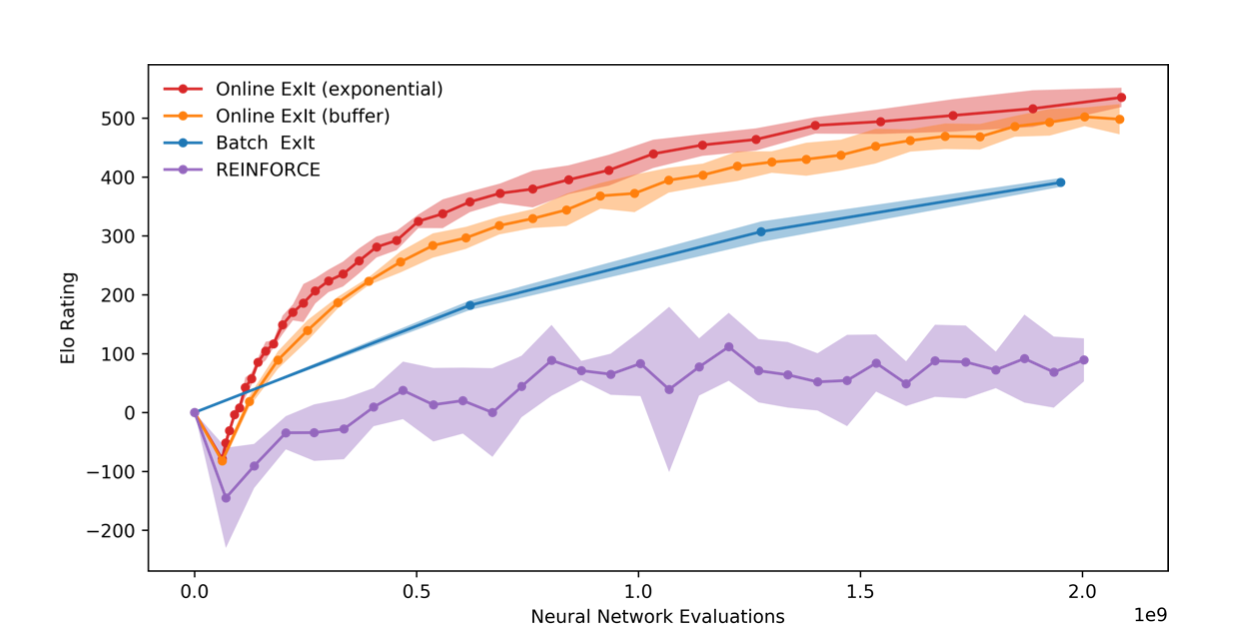
- EXIT vs REINFORCE:
- Learns stronger policies faster
- Shows no sign of instability - policy improves consistently each iter
- Little variation in performance between each training run
- Separating the tree search from generalisation ensures plans don’t overfit to a current opponent since tree search considers multiple possible responses to recommended moves
- Online expert iteration significantly outperforms batch mode
- ‘Exponential dataset’ version of online EXIT marginally stronger than ‘buffer’ version - suggests retaining a larger dataset is useful
Figure 2: Elo ratings of policy gradient network and EXIT networks through training - avg of 5 training runs, shaded areas 90% confidence intervals. Time=number of NN evaluations made
6.2 Comparison of Value and Policy EXIT
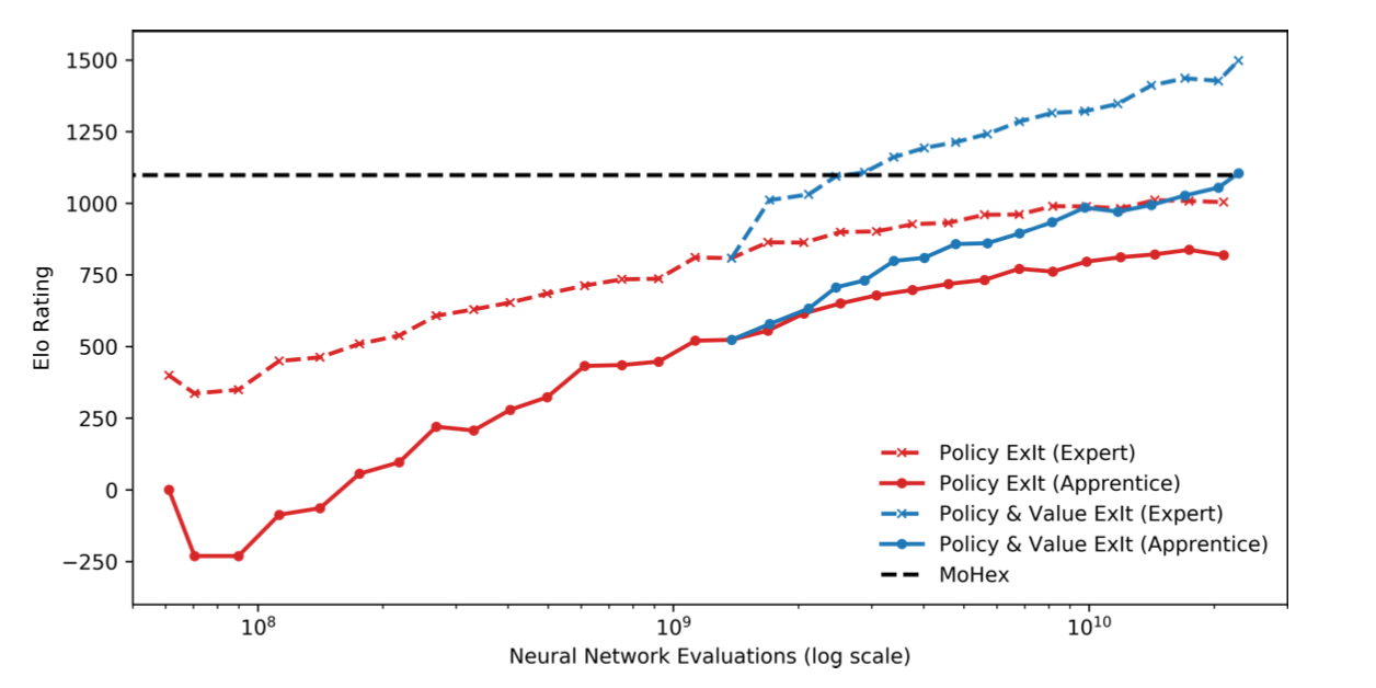
- With large enough datasets, a value network can be learnt to improve expert further
- Ran asynchronous distributed online EXIT using only a policy network until datasets contained ~550k positions
- Used most recent apprentice to add a Monte Carlo value estimate from each position in dataset and trained combined policy and value apprentice, improving quality of expert play significantly
- Then ran EXIT with combined value-and-policy network, creating another ~7.4 million move choices
- For comparison, training run continued without using value estimation for equal time
- Value-and-policy-EXIT significantly outperforms policy-only-EXIT - improved plans from better expert quickly manifest in stronger apprentice
- Importance of expert improvement is clear - later apprentices comfortably outperform earlier training experts
Figure 3: Distributed online EXIT apprentices and experts, with/without neural network value estimation. Black dashed line represents MOHEX’s rating (10k iterations per move).
6.3 Performance Against MoHex
- MoHex versions winners of every Computer Games Olympiad Hex tournament since 2009 (to date of the paper)
- MoHex
- Highly optimised
- Complex hand-made theorem prover
- Calculates provably suboptimal moves to prune
- Improved rollout policy
- Optionally specialised end-game solver
- This model
- Learns tabula rasa
- Without game-specific knowledge apart from rules
- They compare to most recent available at the time (1.0)
- Comparing MoHex to experts with equal wall-clock times difficult since relative speeds hardware dependent
- MoHex CPU-heavy, experts GPU bottlenecked
- In their machine, MoHex ~50% faster
- EXIT (with 10k iterations) won:
- 75.3% of games against 10k iteration-MoHex on default settings,
- 59.3% against 100k iteration-MoHex,
- 55.6% against 4-second-per-move-MoHex (with parallel solver switched on),
- These are than six times slower than their searcher
- Remarkable since training curves in Figure 3 don’t suggest convergence
7 Related Work
- EXIT has several connections to existing RL algorithms given different choices of expert class
- Can recover version of Policy Iteration by using Monte Carlo Search as expert
- Other works also attempted Imitation Learning outperforming the original expert
- Silver et al.: Imitation Learning followed by RL
- Kai-Wei, et al.: Monte Carlo estimates to compute $Q^*(s, a)$ and train apprentice $\pi$ to maximize $\sum_a \pi(a|s)Q^*(s, a)$
- Rollout policy changed each iteration after first to a mix of the most recent apprentice and original expert
- Can see it as blend of an RL algorithm with Imitation Learning: combines Policy Iteration and Imitation Learning
- Neither approach able to improve original expert policy - useful only at the beginning of training
- EXIT, in contrast, creates stronger experts for itself, and can use them throughout training
- AlphaGo Zero (AG0) independently developed version of EXIT and achieved SOTA Go performance, detailed comparison in appendix
- Unlike standard Imitation Learning can apply EXIT to RL problem - doesn’t assume satisfactory expert exists
- Can apply without domain specific heuristics - their experiment used general-purpose algorithm as expert class
8 Conclusion
- New RL algorithm Expert Iteration
- Motivated by dual process theory of human thought
- Decomposes the RL problem by separating generalisation and planning
- Plan on a case-by-case basis
- When MCTS has found significantly stronger plan, then generalise result
- Advantages
- Allows for long-term planning
- Faster learning
- SOTA final performance
- Significantly outperforms a variant of REINFORCE in learning to play Hex
- Competitive with SOTA heuristic search despite tabula rasa training - resultant tree search algorithm beats MoHex 1.0.