PixelCNN

Note: This tutorial was written a while ago. There are several newer pixel-level generative models based on transformers that produce higher quality images. However the basic concepts of masked autoregressive models are still essentially the same so I think the material covered here will still be useful.

Introduction

Generative image modeling is a central problem in unsupervised learning.

However, because images are high dimensional and highly structured, estimating the distribution of natural images is extremely challenging.

One of the most important obstacles in generative modeling is building complex and expressive models that are also tractable and scalable.

One effective approach to tractably model a joint distribution of the pixels in the image is to cast it as a product of conditional distributions.

The factorization turns the joint modeling problem into a sequence problem, where one learns to predict the next pixel given all the previously generated pixels.

Whilst recurrent neural networks are an obvious choice:

We observe that Convolutional Neural Networks (CNN) can also be used as sequence model with a fixed dependency range, by using Masked convolutions. The PixelCNN architecture is a fully convolutional network of fifteen layers that preserves the spatial resolution of its input throughout the layers and outputs a conditional distribution at each location.

\[p(x_{i,R}|x<i)p(x_{i,G}|x<i, x_{i,R})p(x_{i,B}|x<i, x_{i,R}, x_{i,G})\]

In this post we will focus on the PixelCNN architecture. They are simpler to implement and once we have grasped the concepts, we can move on to the PixelRNN architecture in a later post. A repository with the code for this post can be found here.

Contents

• Introduction
• Contents
• Predicting sequences with convolutional networks
• Masking
  • Motivation
  • Masks
  • Implementation
  • Masked convolution
• PixelCNN
• Data
• Losses and metrics
• Training
• Inference
• Putting it all together

Predicting sequences with convolutional networks

[Recurrent models] have a potentially unbounded dependency range within their receptive field. This comes with a computational cost as each state needs to be computed sequentially. One simple workaround is to make the receptive field large, but not unbounded. We can use standard convolutional layers to capture a bounded receptive field and compute features for all pixel positions at once.

From Figure 2 of the paper

Can you explain how a convolutional layer can predict sequences in parallel?

Each pixel of the output (leaving out the very first pixel) can be interpreted as a prediction conditioned on the input pixels above and to the left (leaving out the very last pixel).

Note that the advantage of parallelization of the PixelCNN over the PixelRNN is only available during training or during evaluating of test images. The image generation process is sequential for both kinds of networks, as each sampled pixel needs to be given as input back into the network.

Can you think of any other issues with parallel prediction?

When predicting pixels in parallel, for each pixel the model should only have access to "past" pixels i.e. those above and to the left. Otherwise it would be able to cheat by having access information about elements it is supposed to be predicting.

Masking

Motivation

Masks are adopted in the convolutions to avoid seeing the future context

The $h$ features for each input position at every layer in the network are split into three parts, each corresponding to one of the RGB channels.

When predicting the R channel for the current pixel $x_i$, only the generated pixels left and above of $x_i$ can be used as context.

When predicting the G channel, the value of the R channel can also be used as context in addition to the previously generated pixels.

Likewise, for the B channel, the values of both the R and G channels can be used.

Let us consider an example with 3 feature maps. Step through the animation and try to determine which pixels from input feature maps will contribute to the prediction in each case. For clarity a single arrow is used for the above-and-left pixels to indicate they will be used.

Masks

To restrict connections in the network to these dependencies, we apply a mask …

We use two types of masks that we indicate with mask A and mask B

Mask A is applied only to the first convolutional layer in a PixelRNN and restricts the connections to those neighboring pixels and to those colors in the current pixels that have already been predicted.

On the other hand, mask B is applied to all the subsequent input-to-state convolutional transitions and relaxes the restrictions of mask A by also allowing the connection from a color to itself.

Why do we need to mask the input at position $i,j,c$ to predict the output at $i,j,c$ for the first layer but not for subsequent layers?

We only need to hide the true data. As the diagram shows, the output of the first layer at $i,j,c$, $X1[i,j,c]$ only depends on the previous pixels and not on the pixel $I[i,j,c]$ of the input image $I$, which is the target for position $i,j,c$. Since $X1[i,j,c]$ is therefore only connected to the valid context for position $i,j,c$, it can be used when predicting $X2[i,j,c]$.

Implementation

The masks can be easily implemented by zeroing out the corresponding weights

This is easiest to see if we note that 3x3 convs are used in the Masked Conv layers and that “same” padding is added in order to preserve dimensions. Thus as the kernel slides over the image, the centre of a kernel will be aligned with the pixel whose value is going to be predicted. Like the feature maps are split into 3 corresponding to each colour, the $k \times k \times f_\text{in} \times f_\text{out} $ kernel can be split into 9 of size $k \times k \times (f_\text{in}/3) \times (f_\text{out}/3) $ kernels that map every colour to every other colour.

Applying the masking rules, how will the mask for a $3 x 3$ kernel from each of these groups look like for mask A and mask B? Assume, as noted above, that the centre will be aligned with the “present” pixel.

The dark pixels are 0 and the light pixels are 1. Note for clarity the centre pixel is shown slightly lighter or darker.

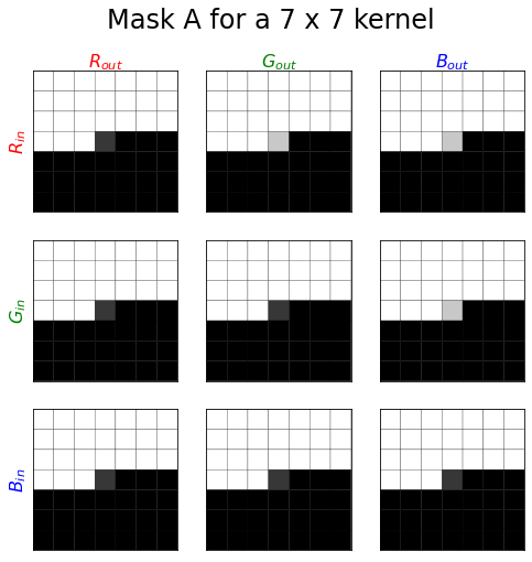
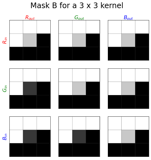
If you group together just the kernel centres, which correspond to the present pixel position you get what looks like an upper triangular matrix. For mask A everything above the diagonal is 1 and for mask B everything above and including the diagonal is 1. Actually it will be a block triangular matrix with blocks of size $f_\text{in}/3 \times f_\text{out}$.

Now try implementing this, keeping in mind these points:

• The mask values will be the same for all the previous pixels.
• The mask values for the present pixel will have an will be matrix of $f_\text{in}/3 \times f_\text{out}$ blocks one or zero blocks that have an upper-triangular form.
• It can be assumed that the kernel size is odd and the image height will be padded by h_k // 2 and width by w_k // 2 to preserve dimensions so that the kernel centre will always correspond to the present pixel

def get_mask(kernel_size, features_in, features_out, mode='B'):
    assert (features_in % 3) == 0, features_in
    assert (features_out % 3) == 0, features_out
    
    # Assume centre of kernel corresponds to present pixel
    # which will be the case if kernel dims are odd
    # and "same" padding is used 
    h, w = kernel_size
    i_cent = h // 2
    j_cent = w // 2
    mask = np.ones((h, w, features_in, features_out))
    
    # all zeros to the left in the centre row
    mask[i_cent, (j_cent + 1):] = 0.
    # all zeros below
    mask[(i_cent + 1):] = 0.
    
    # clr2clr[i, j] indicates whether colour_i
    # in the previous layer is connected to colour_j in present
    # where colours are R,G,B.
    # Entries above the diagonal are always 1 and below always 0
    # since there is no backward flow.
    # For mask B a colour feeds into itself in the next layer
    # so the diagonal entries are 1 but for mask A they are 0
    # meaning that the colour can't feed into itself if mask A is used 
    clr2clr = np.triu(np.ones((3, 3)), k=1 if mode=='A' else 0)
    
    rgb_mask = np.repeat(np.repeat(clr2clr, features_in//3, axis=0), 
                     features_out//3, axis=1)
    
    mask[i_cent, j_cent] = rgb_mask
    
    return mask.astype('float32')

Try plotting the masks from the kernels.

## Parameters to plot the image for mask A shown. Modify to plot different masks
mode = 'A'
k = 7
ksize= (k, k)
f_in = 15
f_out = 24

## Code to plot
m = get_mask(ksize, f_in, f_out, mode)
masks = [[m[:, :, i * f_in//3, j * f_out//3] 
         for j in range(3)]
         for i in range(3)]
masks = [np.pad(i, ([(0, 1)] * 2), constant_values=1)
      for i in 2 * np.stack(masks).reshape([-1, 3, 3])
      ]
masks = np.reshape(masks, ksize + (4, 4))

fig, axes = plt.subplots(3, 3, figsize=(8, 8))
for i, clr_in in enumerate('RGB'):
    for j, clr_out in enumerate('RGB'):
        ax = axes[i, j]
        kernel = deepcopy(m[:, :, i * f_in//3, j * f_out//3]) * 255
        mid = np.floor_divide(kernel.shape, 2)
        mid_val = kernel[mid[0], mid[1]] 
        kernel[mid[0], mid[1]] = 55 if mid_val == 0 else 200
        ax.pcolor(kernel, edgecolor='k', vmin=0, vmax=255, cmap='gray')
        if j == 0:
            ax.set_ylabel('$%s_{in}$'%clr_in, color=clr_in.lower(), fontsize=16)
        if i == 0:
            ax.set_xlabel('$%s_{out}$'%clr_out, color=clr_out.lower(), fontsize=16)
        ax.set_xticks([])
        ax.set_yticks([])
        ax.invert_yaxis()
        ax.xaxis.set_label_position('top')
    
    plt.suptitle(f'Mask {mode} for a {k} x {k} kernel', fontsize=24)

Masked convolution

Let us now implement a masked conv layer. A simple approach is to implement conv layer where the kernel is multiplied with the mask before the convolution step.

class MaskedConv2D(tf.keras.layers.Layer):
    def __init__(self, kernel_size, filters_in, filters, act=None, mode='B'):
        super(MaskedConv2D, self).__init__()
        if isinstance(kernel_size, int):
            self.kernel_size = (kernel_size, kernel_size)
        else:
            self.kernel_size = kernel_size
        self.filters = filters
        self.mode = mode
        if act is not None:
            self.act = tf.keras.layers.Activation(act)

        self.kernel = self.add_weight(name='kernel', shape=(*self.kernel_size, filters_in, self.filters))
        self.bias = self.add_weight(name='bias', shape=(self.filters,))
        mask_kwargs = dict(kernel_size=self.kernel_size, 
                             features_in=filters_in,
                             features_out=self.filters,
                             mode = self.mode)
        self.mask = get_mask(**mask_kwargs)
        
    def call(self, x):
        kernel = self.kernel * self.mask
        out = tf.nn.conv2d(x, kernel, [1, 1, 1, 1], padding='SAME')
        out = tf.nn.bias_add(out, self.bias)
        if hasattr(self, 'act'):
            return self.act(out)
        return out

Note: for simplicity we are passing in the number of input channels. An alternative approach would be to redefine the `build` function so that the mask as well as the weights are initialised when the module is first called so that the number of filters is inferred from the input rather than having to be provided in advance.

PixelCNN

Once masking is understood, the architecture is actually rather simple and does not require many lines of code.

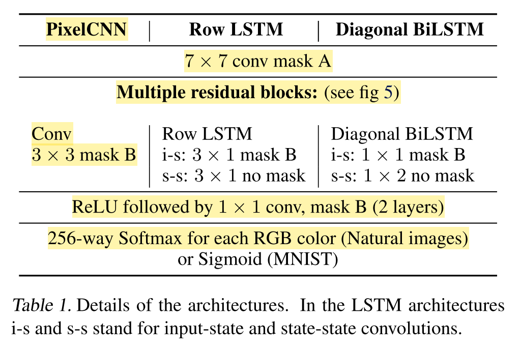
The first layer is a 7 × 7 convolution that uses the mask of type A … The PixelCNN [then] uses convolutions of size 3 × 3 with a mask of type B. The top feature map is then passed through a couple of layers consisting of a Rectified Linear Unit (ReLU) and a 1×1 convolution. For the CIFAR-10 and ImageNet experiments, these layers have 1024 feature maps; for the MNIST experiment, the layers have 32 feature maps. Residual and layer-to-output connections are used across the layers… [Emphasis added]

This is summarised in the following table:

The residual block is as shown below:

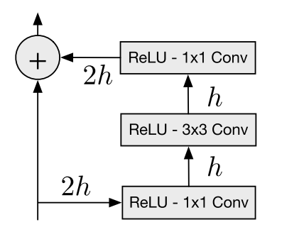
Let us a implement a module PixelCNNResBlock based on the diagram that makes use of the MaskedConv2D layer.

  class PixelCNNResBlock(tf.keras.models.Model):
      def __init__(self, filters_in, filters):
          super(PixelCNNResBlock, self).__init__()
          self.conv_in = MaskedConv2D(1, filters_in, filters, act='relu')
          self.conv_mid= MaskedConv2D(3, filters, filters, act='relu')
          self.conv_out = MaskedConv2D(1, filters, 2 * filters, act='relu')
          
      def __call__(self, x):
          out = self.conv_in(x)
          out = self.conv_mid(out)
          out = self.conv_out(out)
          return x + out

Now we can construct the model. Reshape the output so that it has shape [batch_size, height, width, 3, 256] corresponding to the 256 possible intensities for each colour. We will call this PixelRNN and pass in the residual block as an argument making it possible to reuse the module to also build the recurrent models in the paper later.

class PixelRNN(tf.keras.models.Model):
    def __init__(self, hidden_dim, out_dim, n_layers, pixel_layer):
        super(PixelRNN, self).__init__()
        hidden_dim = hidden_dim * 3
        out_dim = out_dim * 3
        
        self.input_conv = MaskedConv2D(kernel_size=7,
                                       filters_in=3,
                                       filters=2 * hidden_dim,
                                       mode='A')
            
        self.pixel_layer = [pixel_layer(2 * hidden_dim, hidden_dim) for _ in range(n_layers)]
        
        self.output_conv1 = MaskedConv2D(kernel_size=1, 
                                         filters_in=2 * hidden_dim,
                                         filters=out_dim)
        self.output_conv2 = MaskedConv2D(kernel_size=1, 
                                         filters_in=out_dim,
                                         filters=out_dim)
        
        self.final_conv = MaskedConv2D(kernel_size=1, 
                                       filters_in=out_dim,
                                       filters=256 * 3)
    
    def __call__(self, x):
        y = self.input_conv(x) 
        for layer in self.pixel_layer:
            y = layer(y)
            
        y = self.output_conv1(tf.nn.relu(y))
        y = self.output_conv2(tf.nn.relu(y))
        y = self.final_conv(y)
        
        y = tf.reshape(y, tf.concat([tf.shape(y)[:-1], [3, 256]], 0))
        return y

Data

We will use the CIFAR10 dataset and load it into memory using keras. Then we write a simple function get_dataset to create a dataset that does the following

• Normalises the images by 255
• Shuffles the images if training
• Returns a float32 and int32 version of the image where the int32 version is used as the label.

def get_dataset(imgs, batch_size=16, mode='train'):
    def _map_fn(x):
        labels = tf.cast(x, tf.int32)
        imgs = tf.cast(x, tf.float32)
        imgs = imgs / 255.
        return imgs, labels
    ds = tf.data.Dataset.from_tensor_slices(imgs)
    if mode == 'train':
        ds = ds.shuffle(1024)
        ds = ds.repeat(-1)
    ds = ds.map(_map_fn)
    return ds.batch(batch_size)

Losses and metrics

All our models are trained and evaluated on the log-likelihood loss function coming from a discrete distribution. For the multinomial loss function we use the raw pixel color values as categories.

In other words, the model is trained with a softmax cross-entropy loss over the 256 classes for each of red, green and blue.

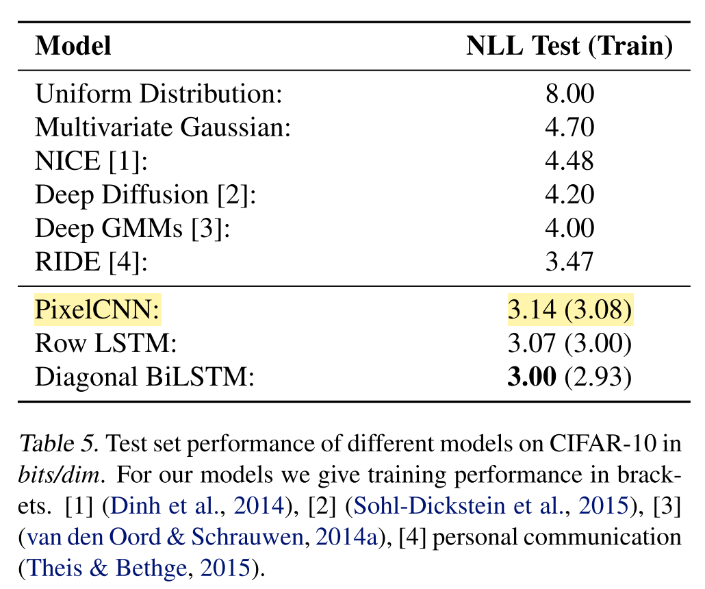
For CIFAR-10 and ImageNet we report negative log-likelihoods in bits per dimension. The total discrete log-likelihood is normalized by the dimensionality of the images (e.g., 32×32×3 = 3072 for CIFAR-10). These numbers are interpretable as the number of bits that a compression scheme based on this model would need to compress every RGB color value (van den Oord & Schrauwen, 2014b; Theis et al., 2015); in practice there is also a small overhead due to arithmetic coding.

How can you derive the negative log-likelihoods (NLL) in bits per dimension from the softmax loss?

The softmax loss for $N$ RGB images of size $H \times W$ is as follows:

\({L_\text{softmax}(I_\text{true}, I_\text{pred})}= \\-\frac{1}{3\cdot NHW}\ln\prod_{i=0}^{N-1}\prod_{x=0}^{H-1}\prod_{y=0}^{W-1}p(x_{i,R}|x_{<i})p(x_{i,G}|x_{<i}, x_{i,R})p(x_{i,B}|x_{<i}, x_{i,R}, x_{i,G})\)

where $x$ is the true intensity.

This is the normalized NLL in nats averaged across the images. Here the $\log$ has base of $e$ whereas to get it in bits per dimension we need to use a base of 2. Since $\log_2(x) = \ln(x) / \ln(2)$, simply dividing the softmax loss by $\ln(2)$ e.g. tf.log(2) or np.log(2) gives you the NLL in bits normalized by the dimensionality of the images and averaged across the images.

Training

RMSProp gives best convergence performance and is used for all experiments. The learning rate schedules were manually set for every dataset to the highest values that allowed fast convergence.

As further details were not provided here about the learning rates, I looked OpenAI’s codebase for PixelCNN++ and found that they used Adam with a learning rate of 0.001 multiplied by 0.999995 after each step so that is what we will use here.

Let us create a Trainer class that will be used to train the model. It will store the model, optimizer, loss function and metrics and have methods to train and evaluate the model. Here is some code to get you started.

class Trainer(object):
    def __init__(self,
                config: dict,   
                 model: tf.keras.models.Model,
                 loss_fn: Union[tf.keras.losses.Loss, Callable],
                 optim: tf.keras.optimizers.Optimizer):
        self.config = config
        self.model = model
        self.loss_fn = loss_fn
        self.optim = optim
        self.ckpt = tf.train.Checkpoint(
            transformer=self.model,
            optimizer=self.optim
        )
        self.trn_writer = tf.summary.create_file_writer(os.path.join(config.log_path, 'train'))
        self.test_writer = tf.summary.create_file_writer(os.path.join(config.log_path, 'test'))
        self.img_writer = tf.summary.create_file_writer(os.path.join(config.log_path, 'imgs'))

Now add the following methods to the class:

• run_model which takes a batch of images and returns the model output and loss
• train_step which takes a batch of images, updates the model weights and returns the loss
• valid_step which takes a batch of images and returns the loss
• evaluate which takes a dataset and returns the average loss

Feel free to add any other methods you think are necessary as well as code to print metrics, add summaries, etc.

    def run_model(self, images, labels):
        predictions = self.model(images)
        batch_size = tf.shape(images)[0]
        # Model can be evaluated on all except for the very first element
        # i.e. the R value of the top left corner pixel
        y_true = tf.reshape(labels, [batch_size, -1])[:, 1:]
        y_pred = tf.reshape(predictions, [batch_size, -1, 256])[:, 1:]
        loss = tf.reduce_mean(self.loss_fn(labels=y_true, logits=y_pred))

        return loss, predictions

    @tf.function
    def train_step(self, images, labels):
        with tf.GradientTape() as tape:
            loss, predictions = self.run_model(images, labels)
        
        grads = tape.gradient(loss, self.model.trainable_variables)
        self.optim.apply_gradients(zip(grads, self.model.trainable_variables))
        itr = self.optim.iterations

        bits_per_dim = loss / tf.math.log(2.)
        with self.trn_writer.as_default():
            tf.summary.scalar('loss', bits_per_dim, itr)
            tf.summary.scalar('lr', self.optim.learning_rate, itr)

        self.optim.learning_rate.assign(
            self.optim.learning_rate * 0.999995
        )

        return bits_per_dim, predictions

    def valid_step(self, images, labels):
        # training=False is only needed if there are layers with different
        # behavior during training versus inference (e.g. Dropout).
        loss, predictions = self.run_model(images, labels)

        return loss, predictions

    @tf.function
    def evaluate(self, dataset: tf.data.Dataset):
        loss = tf.TensorArray(tf.float32, size=tf.cast(len(dataset), tf.int32))
        for idx, (images, labels) in enumerate(dataset):
            loss_, _ = self.valid_step(images, labels)
            idx = tf.cast(idx, tf.int32)
            loss = loss.write(idx, loss_)
        loss = loss.stack()
        bits_per_dim = tf.reduce_mean(loss / tf.math.log(2.))
        with self.test_writer.as_default():
            tf.summary.scalar(
                'bits_per_dim',
                bits_per_dim,
                self.optim.iterations
            )
        return bits_per_dim

Inference

Inference as noted before must be done sequentially. How do think it is done?

• Start with an image consisting of single red pixel samplied uniformly at random from {0, …, 255} and predict a distribution for green at this position.
• Sample from this distribution to get a single value for green.
• Update the image with the green pixel and make a prediction for blue.
• Update the image with the blue pixel and make a prediction for red at the next pixel
• And so on, until the entire image is generated.

Now implement a function generate_images, which given an model and a number of images to generate, repeatedly calls the model to produce an image. The function should use TensorFlow so that it can be run on the GPU and as part of a graph.

Hint: use a tf.while_loop to loop over the HWC pixels of the image and use tf.tensor_scatter_nd_update to update the image.

def generate_images(
                model: tf.keras.models.Model,
                img_dims: Iterable,
                n_images: int=1,
                n_channels: int=3,
                initial_values=None,   
                ) -> tf.Tensor:
    batch_inds = tf.expand_dims(tf.range(n_images), axis=-1)
    # [0, 0, 0, 0, ...], [1, 0, 0, 0, ...], [2, 0, 0, 0, ...], ...
    init_inds = tf.concat(
        [
            batch_inds,
            tf.zeros((n_images, n_channels), dtype='int32')
        ], axis=-1
    )
    if initial_values is None:
        initial_values = tf.random.uniform(shape=(n_images,),
                                                minval=0,
                                                maxval=1,
                                                dtype='float32')
    img = tf.scatter_nd(indices=init_inds,
                        updates=initial_values,
                        shape=(n_images, *img_dims, n_channels))
    # Letting step = 1 lets us omit the condition
    # if (clr + colm + row) > 0;
    # which is used to avoid updating the top left pixel of the first channel
    step = tf.constant(1)
    total_steps = tf.math.reduce_prod(img_dims) * n_channels
    def cond(step, img):
        return tf.less(step, total_steps)
    def body(step, img):
        row = tf.math.floordiv(step, img.shape[2] * n_channels)
        colm = tf.math.floordiv(tf.math.mod(step, img.shape[2] * n_channels), n_channels)
        clr = tf.math.mod(step, n_channels)
        update_inds = tf.concat(
            [
                batch_inds,
                tf.tile([[row, colm, clr]], [n_images, 1])
            ], axis=-1
        )
        # The prediction only depends on the pixels to the left and above
        # so we can be get a bit of speedup by using only the rows
        # upto and including the current row
        result = model(img[:, :row + 1, :, :])
        result_rgb = tf.random.categorical(
            logits=result[:, row, colm, clr], 
            num_samples=1
        )
        result_rgb = tf.cast(tf.squeeze(result_rgb, axis=-1), tf.float32)
        img = tf.tensor_scatter_nd_update(img,
                                        indices=update_inds,
                                        updates=result_rgb / 255.)
        return step + 1, img
    step, img = tf.while_loop(cond, body, [step, img])
    return img

Now we can add a function to Trainer to make image summaries over the course of training.

    @tf.function
    def create_image_samples(self):
        itr = self.optim.iterations
        gen_imgs = generate_images(
            model=self.model,
            img_dims=self.config.img_dims,
        )

        with self.img_writer.as_default():
            tf.summary.image('gen_imgs', tf.cast(gen_imgs * 255, tf.uint8), itr)

Putting it all together

Now that all the components have been implemented we can put them together to train the model. This has been done in the file main.py). The settings are defined in config.yml. Run python main.py to train the model. A GPU is highly recommended as the model takes a long time to train on the CPU.

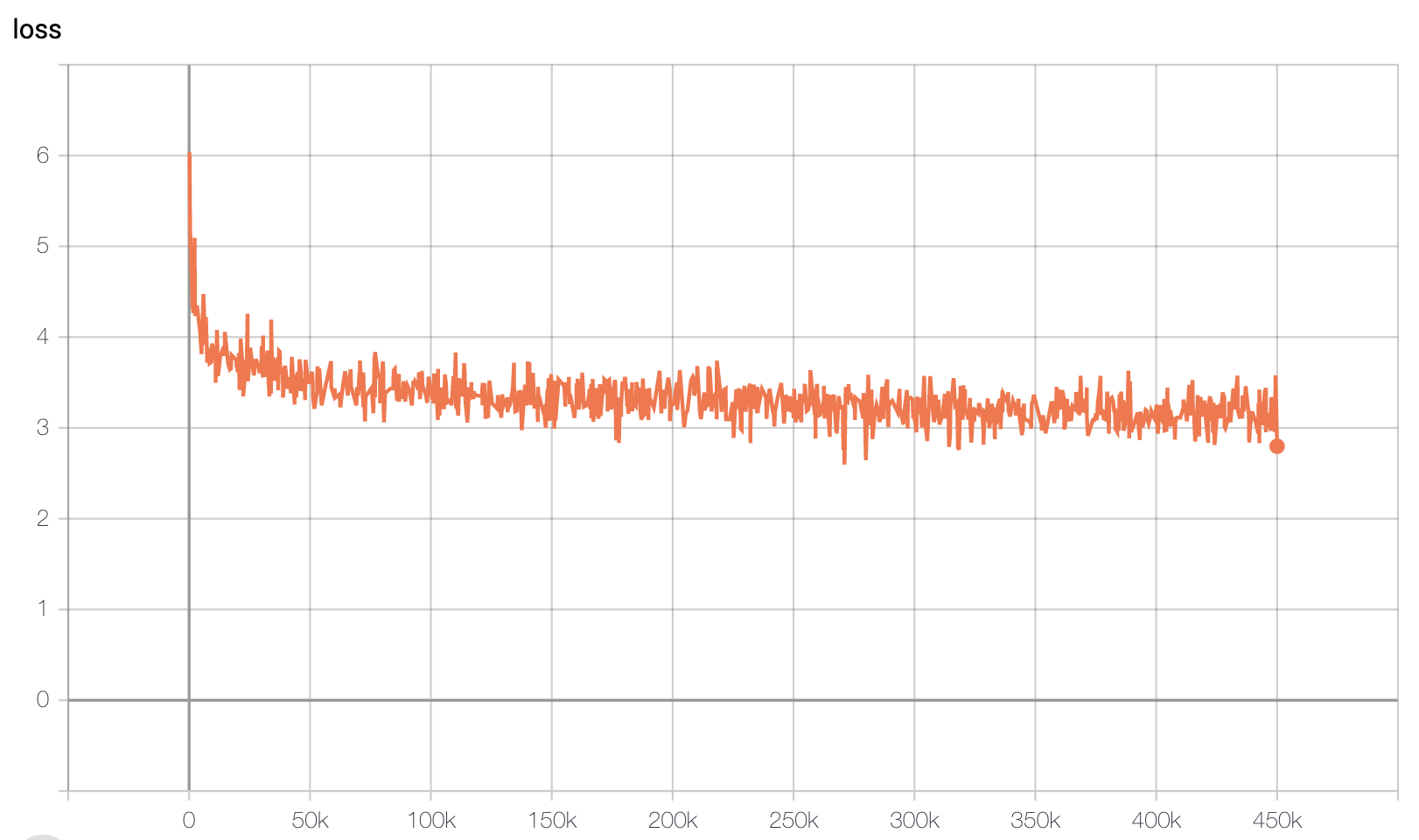
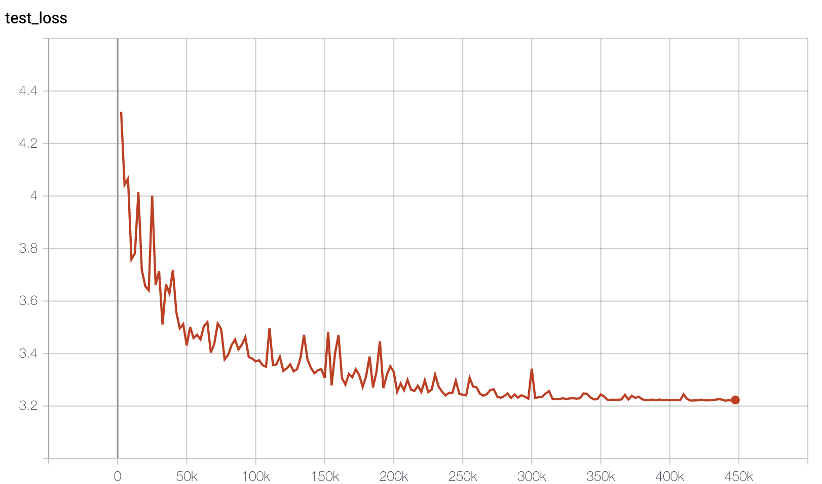
It took over 5 days to run ~450K steps on single GPU for the NLL to get close to the reported values. I stopped it after that as I needed the GPU for other stuff. The test loss went down to about 3.22 which is a bit higher than the reported value in the paper. I have didn’t measure the NLL over the entire training set at a fixed checkpoint and the plot is of the per batch values after each training set. However it can be seen that this converges to a similar level.

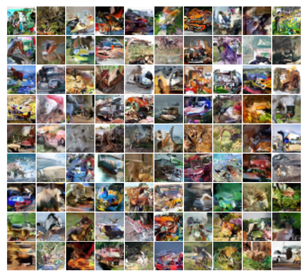
For comparison note that the better performing PixelCNN++ model is said to take around 5 days on 8 GPUs with a batchsize of 16 (so a 8x the number of images per step as used here) to converge it its best value. However image quality seems to improve much sooner. The figure below shows images generated at various points between around 150k and 450k iterations (ordered from left to right top to bottom).

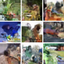
Nevertheless it should be noted that the images don’t match the quality of those that are generated via models such as GANs so don’t be be worried or disappointed if your images don’t seem to resemble anything in the real world. We trade-off model interpretability for quality. Here are examples of images from the models trained in the paper and you can see what they have are plausible patterns of colours but they lack meaningful content.