Transformer Part 1: Build

Introduction

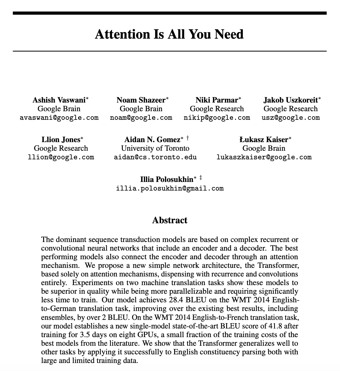
Since its introduction in Attention Is All You Need [1], the Transformer architecture has become very influential and has had successes in many tasks not just in NLP but in other areas like vision. This tutorial is inspired by the approach in The Annotated Transformer [2] which primarily uses text directly quoted from the paper to explain the code (or you could say that it uses code to explain the paper). Differently from [2], which uses PyTorch and adopts a top-down approach to building the model, this tutorial uses Tensorflow along with bottom up approach starting with individual components and gradually putting them together. All quoted sections are from [1].

The code for Parts 1 and 2 of this tutorial can be found in this Colab notebook.

If you notice any problems or mistakes please raise an issue here.

Contents

• Introduction
• Contents
• Motivation
• Architecture
• Attention
  • Scaled Dot-Product Attention
  • Multi-Head Attention
• Position-wise Feed-Forward Networks
• Encoder
• Decoder
• Masking
  • Pad masking
  • Target masking
  • Masked attention
• Inputs and Outputs
• Positional Encoding
• Putting it together
• What’s next
• References

Motivation

Attention mechanisms have become an integral part of compelling sequence modeling and transduction models in various tasks, allowing modeling of dependencies without regard to their distance in the input or output sequences [2, 19]. In all but a few cases [27], however, such attention mechanisms are used in conjunction with a recurrent network.

In this work we propose the Transformer, a model architecture eschewing recurrence and instead relying entirely on an attention mechanism to draw global dependencies between input and output.

Architecture

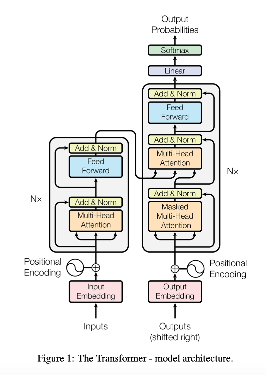
Figure 1 of [1])

Most competitive neural sequence transduction models have an encoder-decoder structure [5, 2, 35]. Here, the encoder maps an input sequence of symbol representations $(x_1,…,x_n)$ to a sequence of continuous representations $z = (z_1,…,z_n)$. Given $z$, the decoder then generates an output sequence $(y_1, …, y_m)$ of symbols one element at a time. At each step the model is auto-regressive [10], consuming the previously generated symbols as additional input when generating the next.

Attention

An attention function can be described as mapping a query and a set of key-value pairs to an output, where the query, keys, values, and output are all vectors. The output is computed as a weighted sum of the values, where the weight assigned to each value is computed by a compatibility function of the query with the corresponding key.

Scaled Dot-Product Attention

We call our particular attention “Scaled Dot-Product Attention” (Figure 2). The input consists of queries and keys of dimension $d$ , and values of dimension $d$ . We compute the dot products of the query with all keys, divide each by $\sqrt{d_k}$, and apply a softmax function to obtain the weights on the values.

In practice, we compute the attention function on a set of queries simultaneously, packed together into a matrix Q. The keys and values are also packed together into matrices K and V . We compute the matrix of outputs as:

\[\text{Attention}(Q, K, V) = \text{softmax}\frac{QK^T}{\sqrt{d_k}} V\]

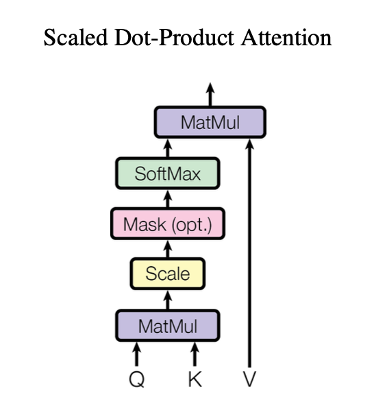
From Figure 2 of [1])

Let us implement the steps in the diagram, not worrying for now about the Mask step. We will call this function scaled_dot_product_attention_temp. Assume there are three inputs query, key and value with final two dimensions (shape[-2:]) N_q, d_k, N_k, d_k, N_v, d_k, where N_k = N_v. Return the final output as well as the attention weights as these are useful for inspecting the model.

def scaled_dot_product_attention_temp(query, key, value, inf=1e9):
    d_k = tf.cast(tf.shape(query)[-1], tf.float32)
    key_transpose = tf.transpose(key,
    tf.concat([tf.shape(key)[:-2], [-1, -2]]))
    qkt = tf.matmul(query, key_transpose)
    alpha = tf.nn.softmax(qkt/tf.sqrt(d_k))
    return tf.matmul(alpha, value), alpha

Multi-Head Attention

Instead of performing a single attention function with $d_\text{model}$-dimensional keys, values and queries, we found it beneficial to linearly project the queries, keys and values h times with different, learned linear projections to $d_k$, $d_k$ and $d_v$ dimensions, respectively. On each of these projected versions of queries, keys and values we then perform the attention function in parallel, yielding $d_v$ -dimensional output values. These are concatenated and once again projected, resulting in the final values

In this work we employ h = 8 parallel attention layers, or heads. For each of these we use dk = dv = dmodel/h = 64. Due to the reduced dimension of each head, the total computational cost is similar to that of single-head attention with full dimensionality.

We can apply scaled_dot_product_attention in parallel across heads, batches and postitions. It can be helpful to track the shapes of the inputs as they get transformed via Multi-Head Attention.

Now we can implement a MultiHeadAttention module which will apply these steps. It will be called on four inputs query, key, value, mask and return a single output.

class MultiHeadAttention(tf.keras.models.Model):
    def __init__(self, dim, num_heads):
        super(MultiHeadAttention, self).__init__()
        self.dim = dim
        self.num_heads = num_heads
        self.transform_query, self.transform_key, self.transform_value = [
            *(tf.keras.layers.Dense(units=dim) for _ in range(3))
        ]
        self.transform_out = tf.keras.layers.Dense(units=dim)

    def split_heads(self, x):
        # x: (B, N, d)
        # (B, N, h, d//h)
        x = tf.reshape(x, (tf.shape(x)[0], -1, self.num_heads, self.dim // self.num_heads))
        # (B, h, N, d//h)
        x = tf.transpose(x, (0, 2, 1, 3))
        return x

    def merge_heads(self, x):
        # x: (B, h, N, d//h)
        # (B, N, h, d//h)
        x = tf.transpose(x, (0, 2, 1, 3))
        # (B, N, d)
        x = tf.reshape(x, (tf.shape(x)[0], -1, self.dim))
        return x

    def call(self, query, key, value, mask):
        # (query=(B, N_q, d), key=(B, N_k, d), value=(B, N_v, d))
        query = self.transform_query(query)
        key = self.transform_key(key)
        value = self.transform_value(value)
        # (query=(B, h, N_q, d//h), key=(B, h, N_k, d//h), value=(B, h, N_v, d//h))
        query, key, value = (self.split_heads(i) for i in [query, key, value])
        # (B, h, N_q, d)
        x, attn = scaled_dot_product_attention(query, key, value, mask)

        x = self.merge_heads(x)
        x = self.transform_out(x)

        return x, attn

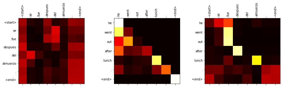
Examples of self-attention and memory attention maps for a translation model (which we will build in the next tutorial):

Position-wise Feed-Forward Networks

[E]ach of the layers in our encoder and decoder contains a fully connected feed-forward network, which is applied to each position separately and identically. This consists of two linear transformations with a ReLU activation in between. FFN(x) = max(0, xW1 + b1 )W2 + b2 (2) While the linear transformations are the same across different positions, they use different parameters from layer to layer. Another way of describing this is as two convolutions with kernel size 1. The dimensionality of input and output is dmodel = 512, and the inner-layer has dimensionality dff =2048.

Let us implement a class FeedForward. It should be an instance of tf.keras.models.Model and take a single input.

Implementation details:

• Input of of size B x N x D=512
• Position-wise meaning that this is treated like a batch of B*N vectors of dimension D
• A two layer neural network:
  • Hidden dimension of 2048
  • ReLU activation after first layer
  • Output dimension of 512

class FeedForward(tf.keras.models.Model):
    def __init__(self, hidden_dim, output_dim):
        super(FeedForward, self).__init__()
        self.dense1 = tf.keras.layers.Dense(hidden_dim,
                                            activation='relu')
        self.dense2 = tf.keras.layers.Dense(output_dim)

    def call(self, x):
        x = self.dense2(self.dense1(x))
        return x

Encoder

The encoder is composed of a stack of N = 6 identical layers. Each layer has two sub-layers. The first is a multi-head self-attention mechanism, and the second is a simple, position- wise fully connected feed-forward network. We employ a residual connection [11] around each of the two sub-layers, followed by layer normalization [1]. That is, the output of each sub-layer is LayerNorm(x + Sublayer(x)), where Sublayer(x) is the function implemented by the sub-layer itself. To facilitate these residual connections, all sub-layers in the model, as well as the embedding layers, produce outputs of dimension dmodel = 512.

Let us start by building the Sublayer block shown below. One way to implement it is to implement a ResidualLayer module in which the Dropout, Add & Norm and the residual connection are contained in a single block. The model receives the input and output to the sublayer which the sublayer might be the FeedForward and MultiHeadedAttention blocks. These are the key details:

• Add dropout to the sublayer output
• Followed by LayerNorm
• Residual connection by adding the sublayer input
• All layers have same output dimensions of d_model

Hint: sublayers can have had an arbitrary number of inputs for example, query, key and value and mask(s) are required for the multi-headed attention. Think about how to handle that.

class ResidualLayer(tf.keras.layers.Layer):
    def __init__(self, dropout=0.0):
        super(ResidualLayer, self).__init__()
        self.use_dropout = dropout > 0
        if self.use_dropout:
            self.dropout_layer = tf.keras.layers.Dropout(dropout)
        self.layer_norm = tf.keras.layers.LayerNormalization(epsilon=1e-6)

    def call(self, skip, out, training=True):
        if self.use_dropout:
            out = self.dropout_layer(out, training=training)
        return self.layer_norm(skip + out, training=training)

Now we can use this component block to construct a module EncoderBlock, which will be the building block of the encoder:

• Multi-Head Attention sublayer block with self-attention so input is used as key, query and value
• Followed by FeedForward sublayer block
• Encoder masking will be used in the attention block

class EncoderBlock(tf.keras.models.Model):
    def __init__(self, dim, ff_dim, num_heads, dropout=0.0):
        super(EncoderBlock, self).__init__()
        self.attn_block = MultiHeadAttention(dim, num_heads)
        self.res1 = ResidualLayer(dropout)
        self.ff_block = FeedForward(hidden_dim=ff_dim, output_dim=dim)
        self.res2 = ResidualLayer(dropout)

    def call(self, query, key, value, mask, training=True):
        x, attn = self.attn_block(query, key, value, mask, training=training)
        skip = x = self.res1(skip=query, out=x, training=training)
        x = self.ff_block(x)
        x = self.res2(skip=skip, out=x, training=training)
        return x, attn

Finally we can put together the Encoder, which consists of a stack of N encoder blocks.

class Encoder(tf.keras.models.Model):
    def __init__(self, dim, ff_dim, num_heads, num_blocks, dropout=0.0):
        super(Encoder, self).__init__()
        self.blocks = [
            EncoderBlock(dim, ff_dim, num_heads, dropout=dropout)
            for _ in range(num_blocks)
        ]

    def call(self, query, mask, training=True):
        attn_maps = []
        for block in self.blocks:
            query, attn = block(
                          query=query, key=query, value=query,
                          mask=mask, training=training)
            attn_maps.append(attn)
        return query, attn_maps

Decoder

The decoder is also composed of a stack of N = 6 identical layers. In addition to the two sub-layers in each encoder layer, the decoder inserts a third sub-layer, which performs multi-head attention over the output of the encoder stack. Similar to the encoder, we employ residual connections around each of the sub-layers, followed by layer normalization.

Let us write a DecoderBlock. The decoder block consists of the following:

• The two sublayers in the encoder block.
• An additional attention layer which has key and value inputs from the encoder.

Hint: it will be very similar to EncoderBlock but remember that the inputs to the final AttentionBlock will be different. Can you reuse EncoderBlock?

class DecoderBlock(tf.keras.models.Model):
    def __init__(self, dim, ff_dim, num_heads, dropout=0.0):
        super(DecoderBlock, self).__init__()
        self.self_attn_block = MultiHeadAttention(dim, num_heads)
        self.res = ResidualLayer(dropout=dropout)
        self.memory_block = EncoderBlock(dim, ff_dim, num_heads, dropout=dropout)

    def call(self, query, key, value, decoder_mask, memory_mask, training=True):
        # if not self.skip_attn:
        x, self_attn = self.self_attn_block(query, query, query, decoder_mask, training=training)
        x = self.res(skip=query, out=x, training=training)
        x, attn = self.memory_block(x, key, value, memory_mask, training=training)
        return x, self_attn, attn

The decoder network will be very similar to the encoder except that it will receive two different mask inputs, one for self-attention and the other for the encoder outputs.

class Decoder(tf.keras.models.Model):
    def __init__(self, dim, ff_dim, num_heads, num_blocks, dropout=0.0):
        super(Decoder, self).__init__()
        self.blocks = [
            DecoderBlock(dim, ff_dim, num_heads, dropout=dropout)
            for i in range(num_blocks)
        ]

    def call(self, query, memory, decoder_mask, memory_mask, training=True):
        self_attn_maps = []
        memory_attn_maps = []
        for block in self.blocks:
            query, self_attn, memory_attn = block(
                      query=query, key=memory, value=memory,
                      decoder_mask=decoder_mask,
                      memory_mask=memory_mask,
                      training=training)
            self_attn_maps.append(self_attn)
            memory_attn_maps.append(memory_attn)

        return query, self_attn_maps, memory_attn_maps

Masking

Two kinds of masks are used to prevent information flow from some sequence positions.

You can plot the masks generated below after squeezing the dimensions of size 1, using the following code:

def plot_mask(mask):
    plt.pcolormesh(mask, cmap='gray', vmin=0, vmax=1, edgecolors='gray')
    plt.gca().invert_yaxis()
    plt.axis('off')

Pad masking

This type of masking is not specific to the Transformer and is not discussed in the paper but used in practice. Padding sequences to the same length allows us to batch together sequences of different lengths. However this is only an engineering requirement and we don’t actually want the model to use the padding elements. The solution is to mask all the positions that have a padding symbol.

Implement a SequenceMask class that does the following:

• Given an integer pad symbol or set of such symbols, produces a boolean tensor where which is False at a location if the value is any of the pad symbols otherwise True
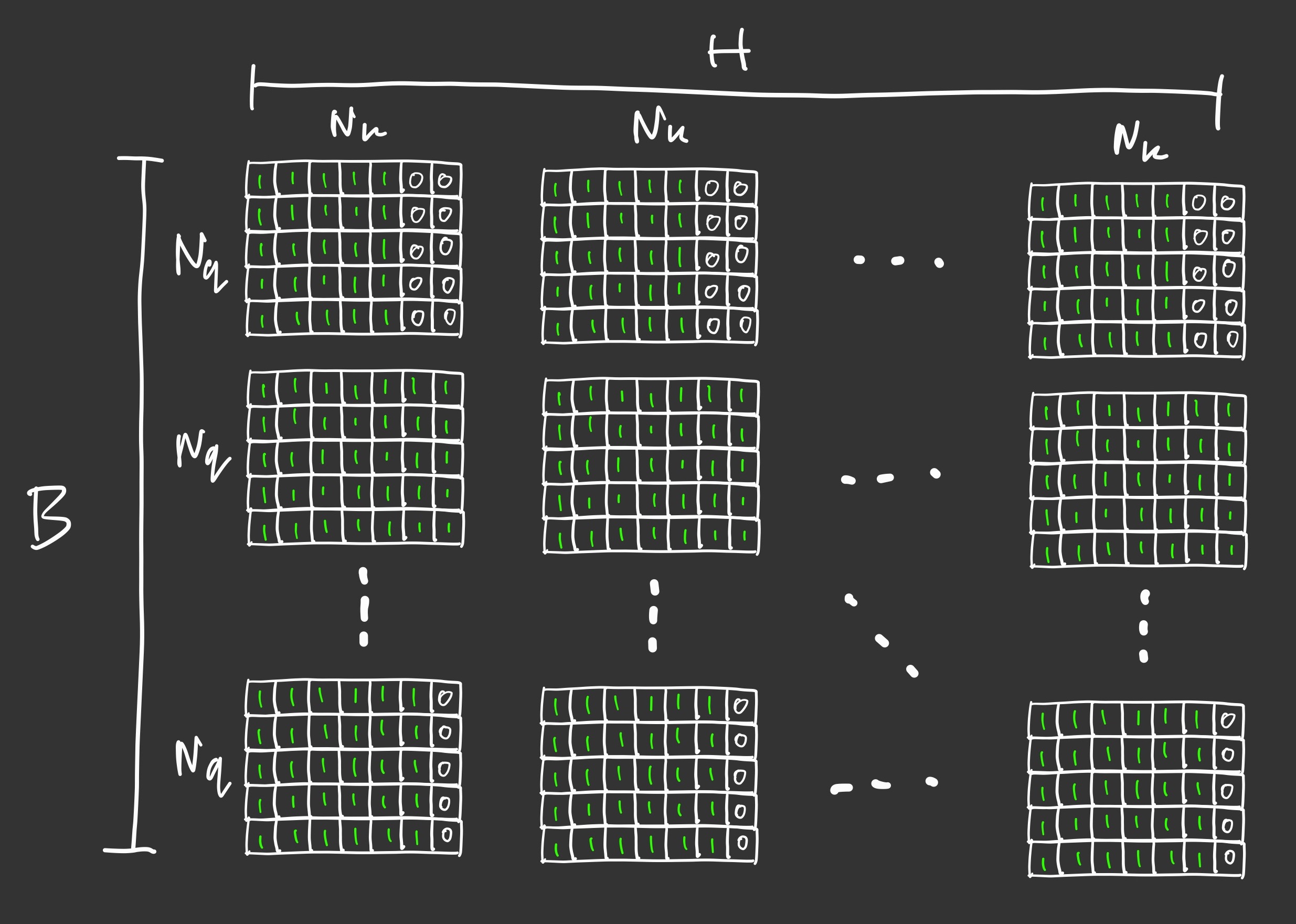
• Returns a (batch_size, 1, 1, sequence_length) tensor that is suitable for using in scaled_dot_product_attention
• When applied to a query of length $N_q$ and key of length $N_k$ this is equivalent to a $N_q \times N_k$ sequence-specific mask for each batch element but shared by all the attention heads, as shown in the figure below:

class SequenceMask:
    def __init__(self, pad):
        self.pad = pad

    def __call__(self, x):
        # Disregards padded elements
        # x: (B, N)
        if isinstance(self.pad, int):
            mask = tf.not_equal(x, self.pad)
        else:
            mask = tf.reduce_all(tf.not_equal(x[..., None], self.pad), axis=-1)
        # Same mask for every position
        # (B, 1, 1, N)
        return mask[:, None, None]

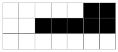
The sequence masks for tf.stack([[1, 2, 3, 4, 5, 0, 0], [1, 2, 0, 0, 0, 0, 0], [1, 2, 3, 4, 5, 6, 7]]) and pad=0:

Target masking

Since we train all the target positions in parallel, the model has access to elements from the “future” and we need to prevent information flowing from later to earlier positions.

We also modify the self-attention sub-layer in the decoder stack to prevent positions from attending to subsequent positions. This masking, combined with fact that the output embeddings are offset by one position, ensures that the predictions for position $i$ can depend only on the known outputs at positions less than $i$.

Implement a subsequent_mask function that for sequence_length=N returns an $N \times N$ tensor, mask where, mask[i, j] = i <=j

This will be used for self-attention only and when applied to a query of length $N$ will broadcast to a $N \times N$ sequence-agnostic mask shared across all the batch elements and attention heads, as shown below:

Hint: use tf.linalg.band_part.

def subsequent_mask(seq_length):
    # (N, N)
    # lower_triangular matrix
    future_mask = tf.linalg.band_part(
        tf.ones((seq_length, seq_length)),
        -1, 0)
    future_mask = tf.cast(future_mask, tf.bool)
    return future_mask

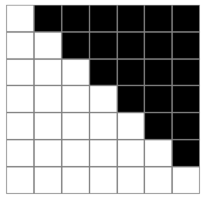
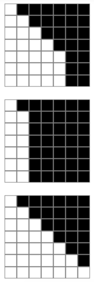
The result for subsequent_mask(7):

Now write a TargetMask class that inherits from SequenceMask does the following when called:

• Creates a future mask for the input sequence
• Creates a sequence mask for the input
• Combines these so that combined_mask[:, j] = False if position j is padding else combined_mask[:, j] = future_mask[i, j]
• Returns a (batch_size, 1, sequence_length, sequence_length) tensor that is suitable for using in scaled_dot_product_attention

class TargetMask(SequenceMask):
    def __call__(self, x):
        # Disregards "future" elements and any others
        # which are padded
        # x: (B, N)
        # (B, 1, N)
        pad_mask = super().__call__(x)
        seq_length = tf.shape(x)[-1]
        # Mask shared for same position across batches
        # (N, N)
        future_mask = subsequent_mask(seq_length)
        # (B, 1, 1, N) & (N, N) -> (B, 1, N, N)
        mask = tf.logical_and(pad_mask, future_mask)
        return mask

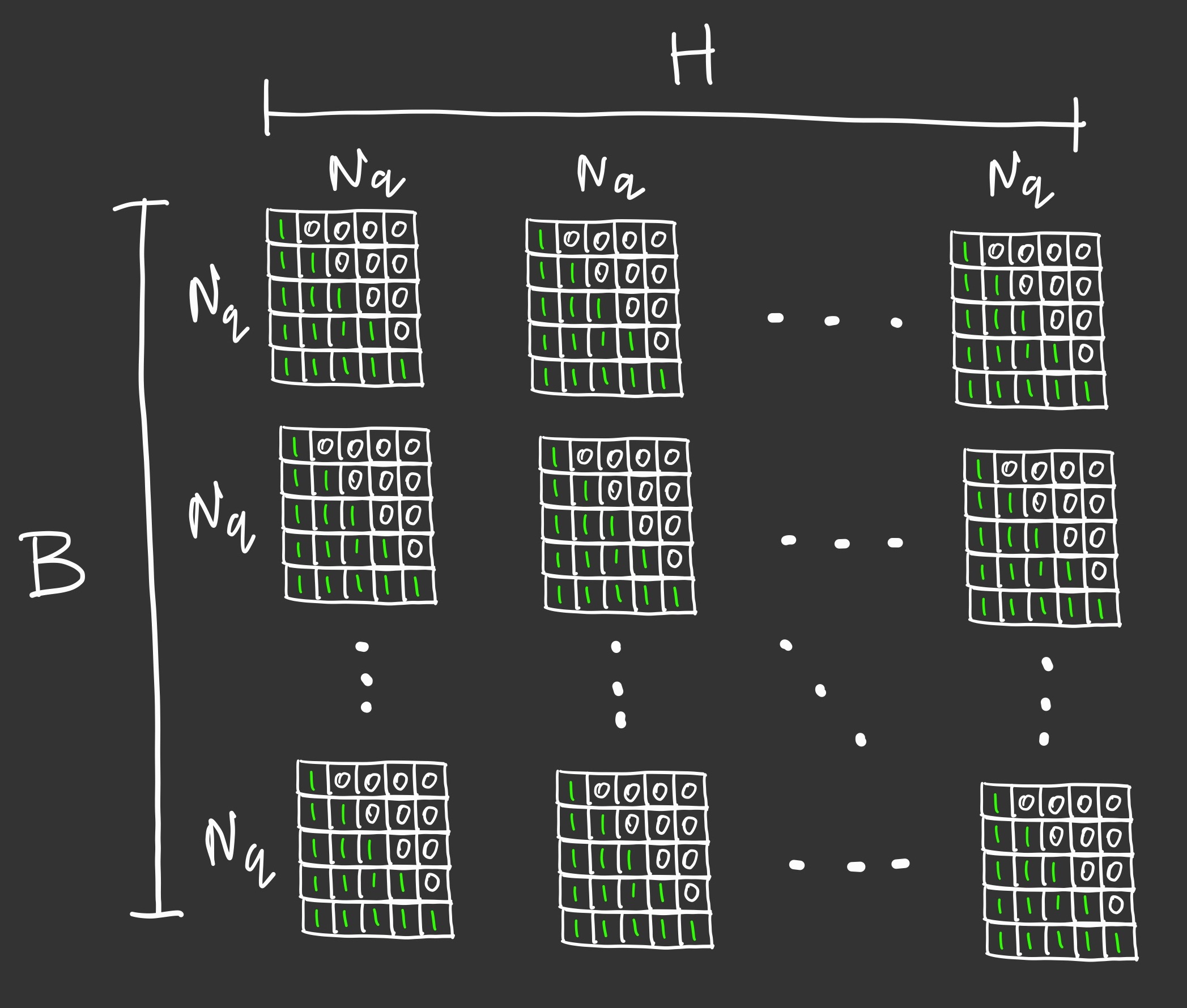
The target masks for tf.stack([[1, 2, 3, 4, 5, 0, 0], [1, 2, 0, 0, 0, 0, 0], [1, 2, 3, 4, 5, 6, 7]]) and pad=0:

Masked attention

In attention layers, the attention weights should be 0 for the padding elements so that other elements don’t attend to these elements.

We need to prevent leftward information flow in the decoder to preserve the auto-regressive property. We implement this inside of scaled dot-product attention by masking out (setting to $-\infty$) all values in the input of the softmax which correspond to illegal connections.

One way to handle masking is to set the positions where mask=False to a negative value with large magnitude such that its softmax score is almost zero and has negligible effect on the scores of the values where mask=True.

def scaled_dot_product_attention_temp(query, key, value, inf=1e9):
    d_k = tf.cast(tf.shape(query)[-1], tf.float32)
    key_transpose = tf.transpose(key,
    tf.concat([tf.shape(key)[:-2], [-1, -2]]))
    qkt = tf.matmul(query, key_transpose)
    alpha = tf.nn.softmax(qkt/tf.sqrt(d_k))
    return tf.matmul(alpha, value), alpha

Inputs and Outputs

[W]e use learned embeddings to convert the input tokens and output tokens to vectors of dimension $d_\text{model}$. We also use the usual learned linear transformation and softmax function to convert the decoder output to predicted next-token probabilities. In our model, we share the same weight matrix between the two embedding layers and the pre-softmax linear transformation, similar to [30]. In the embedding layers, we multiply those weights by $\sqrt{d_\text{model}}$

A simple approach to share the weights is to implement an ScaledEmbedding layer using tf.keras, then get the weight from this layer and matrix multiply to generate the input to the softmax. Alternatively we can skip weight sharing and just use a dense layer for the output.

Accordingly let implement us implement a ScaledEmbedding that takes as input a num_tokens length vector.

Hint: you can multiply the output by $\sqrt{d_\text{model}}$ instead of the weights.

class ScaledEmbedding(tf.keras.layers.Layer):
    def __init__(self, num_tokens, dim):
        super(ScaledEmbedding, self).__init__()
        self.embed = tf.keras.layers.Embedding(
                input_dim=num_tokens,
                output_dim=dim
        )
        self.dim = tf.cast(dim, tf.float32)

    def call(self, x):
        return tf.sqrt(self.dim) * self.embed(x)

If we want to share weights, we can do as follows:

tf.matmul(x, embed_layer.weights[0], transpose_b=True)

Positional Encoding

Since our model contains no recurrence and no convolution, in order for the model to make use of the order of the sequence, we must inject some information about the relative or absolute position of the tokens in the sequence. To this end, we add “positional encodings” to the input embeddings at the bottoms of the encoder and decoder stacks. The positional encodings have the same dimension dmodel as the embeddings, so that the two can be summed.

In this work, we use sine and cosine functions of different frequencies:

\[PE_{(\text{pos},2i)} = \sin(\text{pos}/10000^{2i/d_\text{model}})\] \[PE_{(\text{pos},2i+1)} = \cos(\text{pos}/10000^{2i/d_\text{model}})\]

where $\text{pos}$ is the position and $i$ is the dimension.

[W]e apply dropout to the sums of the embeddings and the positional encodings in both the encoder and decoder stacks

Let us implement a PostionalEncoding layer as follows:

• Receives as input a batch of embeddings size $(B, N, d_\text{model})$
• Generates the positional encoding according to the equations above
• Adds these to the input and applies dropout to the result

class PositionalEncoding(tf.keras.models.Model):
    def __init__(self, dim, dropout=0.0):
        super(PositionalEncoding, self).__init__()
        # (D / 2,)
        self.range = tf.range(0, dim, 2)
        self.dim = tf.cast( 1 / (10000 ** (self.range / dim)), tf.float32)
        self.use_dropout = dropout > 0
        if self.use_dropout:
            self.dropout_layer = tf.keras.layers.Dropout(dropout)

    def call(self, x, training=True):
        # x: (B, N, D)
        # (N,)
        length = tf.shape(x)[-2]
        pos = tf.cast(tf.range(length), tf.float32)
        # (1, N) / (D / 2, 1) -> (D / 2, N)
        inp = pos[None] * self.dim[:, None]
        sine = tf.sin(inp)
        cos = tf.cos(inp)
        # (D, N)
        enc = tf.dynamic_stitch(
            indices=[self.range, self.range + 1],
            data=[sine, cos]
        )
        # (N, D)
        enc = tf.transpose(enc, (1, 0))[None]

        if self.use_dropout:
            return self.dropout_layer(x + enc, training=training)
        return x + enc

To get a positional encoding of shape [length, dim] that you can plot, call PositionalEncoding(dim)(tf.zeros((1, length, dim))).numpy().squeeze(). (With a zeros input and zero dropout just the positional encoding is returned).

Here we can see for a few positions how for each dimension, the positional encoding tends to vary at each position helping to differentiate between the positions

plt.figure(figsize=(12, 8))
d_model = 32
length = 128
pe = PositionalEncoding(d_model)(tf.zeros([1, 128, d_model])).numpy().squeeze()
plt.plot(np.arange(length), pe[:, 8:16]);

In the plots below we plot the positional encodings as:

d_model, length-sized vectors, showing how at each dimension the value at each position varies

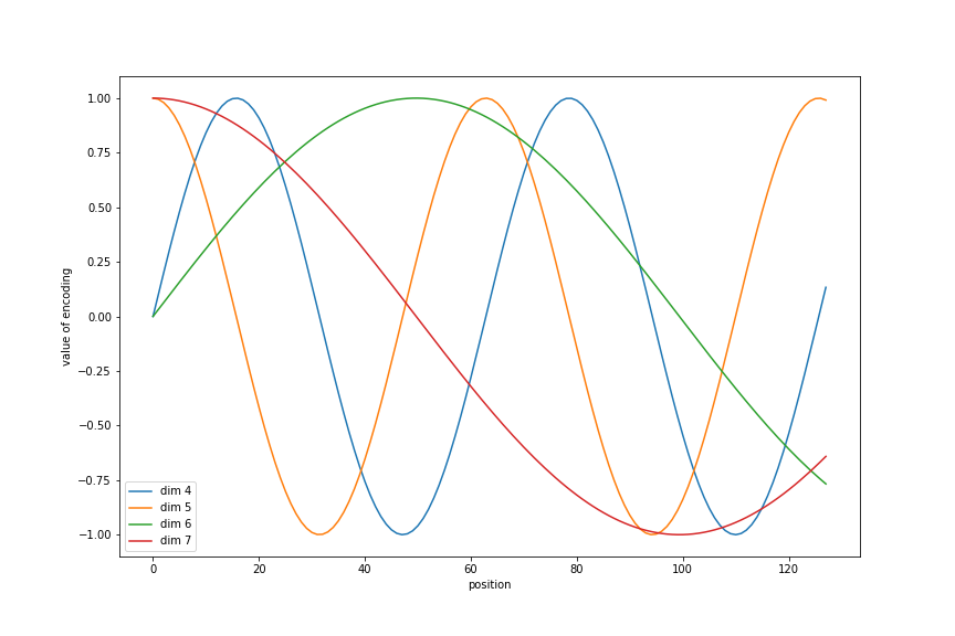
Here we see the sinusoids for a few positions:

fig = plt.figure(figsize=(12, 8))
d_model = 16
length = 128
pe = PositionalEncoding(d_model)(tf.zeros([1, 128, d_model])).numpy().squeeze()
plt.plot(np.arange(length), pe[:, 4:8]);
plt.legend(["dim %d"%p for p in range(4, 8)])
plt.xlabel('position')
plt.ylabel('dimension')

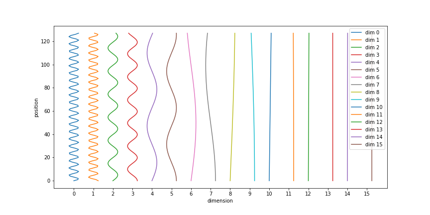
In this figure all the positions are plotted

fig = plt.figure(figsize=(12, 6))
d_model = 16
length = 128
pe = PositionalEncoding(d_model)(tf.zeros([1, length, d_model])).numpy().squeeze()
# add an offset to so that 
offset = 4 * np.arange(d_model) 
# plot with orientation consistent with the [length, d_model] shape of the inputs
plt.plot((pe + offset), np.arange(length));
plt.xticks(offset);
fig.axes[0].set_xticklabels(offset // 4);
plt.xlabel('dimension')
plt.ylabel('position')
plt.legend(["dim %d"%p for p in range(length)], loc='upper right')

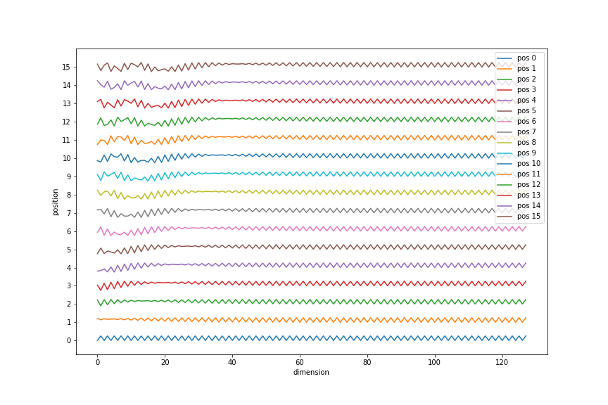
2/ length, d_model-sized vectors, which lets us see how each position can be represented as a different sinusoid

fig = plt.figure(figsize=(12, 8))
d_model = 128
length = 16
pe = PositionalEncoding(d_model)(tf.zeros([1, length, d_model])).numpy().squeeze()
offset = 4 * np.arange(length)
plt.plot(np.arange(d_model), (pe + offset[:, None]).T);
plt.yticks(offset);
fig.axes[0].set_yticklabels(offset // 4);
plt.xlabel('dimension')
plt.ylabel('position')
plt.legend(["pos %d"%p for p in range(length)])

Putting it together

Now using all the classes and functions that we have written we can build a transformer. Write a Transformer class that is initialised with the following arguments:

num_src_tokens	Number of tokens in the input / source dataset
num_tgt_tokens	Number of tokens in the target dataset
model_dim	Same as d_model
num_heads	Number of attention heads in MultiHeadAttention
dropout	Value between 0 and 1 indicating fraction of units to drop in dropout layers
ff_dim	Number of hidden dimensions for the FeedForward block
num_encoder_blocks	Number of EncoderBlock modules to use in Encoder
num_decoder_blocks	Number of DecoderBlock modules to use in Decoder
share_embed_weights	Whether to share the embedding weights for source and target, only applicable if num_src_tokens=num_tgt_tokens
share_softmax_weights	Whether to share the weights between the output layer and the target embeddings

This module will be called with the following inputs:

• Batch of source sequences as tokens
• Batch of target sequences as tokens
• Mask for the source sequence
• Mask for the target sequence
• A boolean training

It will have the following methods

• encode which only takes the inputs needed to generate the output Encoder
  • Batch of source sequences as tokens
  • Mask for the source sequence
  • A boolean training
• decode which assumes that an encoded sequence is available and takes only the inputs need to generate the final classification logits
  • Batch of target sequences as tokens
  • The output from the encode
  • Mask for the source sequence (to use for masking the encoder’s output)
  • Mask for the target sequence
  • A boolean training
• call which calls encode and decode and returns the final logits

class Transformer(tf.keras.models.Model):
    def __init__(self,
                 num_tokens,
                 num_tgt_tokens,
                 model_dim=256,
                 num_heads=8,
                 dropout=0.1,
                 ff_dim=2048,
                 num_encoder_blocks=6,
                 num_decoder_blocks=6,
                 share_embed_weights=False,
                 share_output_weights=False):
        super(Transformer, self).__init__()
        self.share_embed_weights = share_embed_weights
        self.share_output_weights = share_output_weights
        self.input_embedding = ScaledEmbedding(num_tokens, model_dim)
        self.enc_pos_encoding = PositionalEncoding(model_dim, dropout=dropout)
        self.dec_pos_encoding = PositionalEncoding(model_dim, dropout=dropout)

        if not self.share_embed_weights:
            self.target_embedding = ScaledEmbedding(num_tgt_tokens, model_dim)

        self.encoder = Encoder(dim=model_dim,  # 256
                               ff_dim=ff_dim,  # 2048
                               num_heads=num_heads,  # 8
                               dropout=dropout,
                               num_blocks=num_encoder_blocks)

        self.decoder = Decoder(dim=model_dim,  # 256
                               ff_dim=ff_dim,  # 2048
                               num_heads=num_heads,  # 8
                               dropout=dropout,
                               num_blocks=num_decoder_blocks)
        if not self.share_output_weights:
            #TODO: I think need to scale this
            self.output_layer = tf.keras.layers.Dense(units=num_tgt_tokens)

    def encode(self, x, src_mask, training=True):
        x = self.input_embedding(x)
        x = self.enc_pos_encoding(x, training=training)
        memory, attn = self.encoder(x, mask=src_mask, training=training)
        return memory, attn

    def decode(self, y, memory, src_mask, tgt_mask, training=True):
        if self.share_embed_weights:
            y = self.input_embedding(y)
        else:
            y = self.target_embedding(y)
        y = self.dec_pos_encoding(y, training=training)
        out, self_attn, attn = self.decoder(y, memory,
                           memory_mask=src_mask,
                           decoder_mask=tgt_mask,
                           training=training)
        if not self.share_output_weights:
            logits = self.output_layer(out)
        else:
            # This works because this is called only after
            # target_embedding is called so the weights will
            # have been created
            if not self.share_embed_weights:
                embed = self.target_embedding
            else:
                embed = self.input_embedding
            logits = tf.matmul(out, embed.weights[0], transpose_b=True)
        return logits, self_attn, attn

    def call(self, x, y, src_mask, tgt_mask, training=True):
        memory, enc_attn = self.encode(x, src_mask, training=training)
        logits, dec_self_attn, dec_attn = self.decode(y, memory,
                        src_mask=src_mask,
                        tgt_mask=tgt_mask,
                        training=training)
        attention = dict(
            enc=enc_attn,
            dec_self=dec_self_attn,
            dec_memory=dec_attn
        )
        return logits, attention

What’s next

We have built a Transformer but we are not done yet. The paper introduces some approaches to train the model and we need to implement those and we need to write to code to prepare the data and to process the outputs. In Part 2 we will learn how to do all of these and train a translation model.

References

1. Attention Is All You Need
2. The Annotated Transformer