Transformer Part 2: Train a Translation Model
Introduction
In Part 1 of the tutorial we learned how to how build a transformer model. Now it is time to put it into action. There are lots of things we can do with a transformer but we will start off with a machine translation task to translate from Spanish to English.
The code for Parts 1 and 2 of this tutorial can be found in this Colab notebook.
If you notice any problems or mistakes please raise an issue here.
Acknowledgements
This tutorial like the previous was inspired by The Annotated Transformer.
It also borrows and adapts code for data preparation, saving, plotting and other utility functions from the following sources:
- TensorFlow’s RNN-based translation tutorial: https://www.tensorflow.org/tutorials/text/nmt_with_attention
- TensorFlow’s Transformer tutorial: https://www.tensorflow.org/tutorials/text/transformer
Contents
- Introduction
- Contents
- Optimisation
- Loss
- Configuration
- Data
- Metrics
- Set up the experiment
- Train
- Inference
- Attention maps
- What’s next
- References
Optimisation
We used the Adam optimizer [20] with $\beta_1 = 0.9$, $\beta_2 = 0.98$ and $\epsilon = 10$.
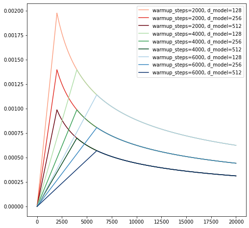
We varied the learning rate over the course of training, according to the formula:
\[\text{lrate}=d_\text{model}^{−0.5} \cdot \min(\text{step_num}^{−0.5}, \text{step_num}\cdot\text{warmup_steps}^{−1.5})\]This corresponds to increasing the learning rate linearly for the first warmup_steps training steps, and decreasing it thereafter proportionally to the inverse square root of the step number. We used $\text{warmup_steps} = 4000$.
Create a custom schedule using tf.keras.optimizers.schedules.LearningRateSchedule. It should have the following methods:
__init__ |
Initialise the hyperparameters |
__call__ |
Receives a value step as input and returns the learning rate according to the above equation |
class LearningRateScheduler(tf.keras.optimizers.schedules.LearningRateSchedule):
    def __init__(self, d_model, warmup_steps):
        self._d_model = d_model
        self._warmup_steps = warmup_steps
        self.d_model_term = d_model ** (-0.5)
        self.warmup_term = warmup_steps ** (-1.5)

    def get_config(self):
        return dict(d_model=self._d_model, warmup_steps=self.warmup_steps)

    def __call__(self, step):
        step_term = tf.math.minimum(step ** (-0.5), step * self.warmup_term)
        return self.d_model_term * step_term
Try plotting the learning rate curve for a few different values of d_model and warmup_steps to get a sense of how it evolves over time.
plt.figure(figsize=(8, 8))
t = tf.range(20000, dtype=tf.float32)
d_model = np.stack([128, 256, 512])
warmup_steps = [2000, 4000, 6000]

for cmap, w in zip(['Reds', 'Greens', 'Blues'], warmup_steps):
  cm = plt.cm.get_cmap(cmap)
  for i, d in enumerate(d_model, 1):

    lr_wd = LearningRateScheduler(
      d_model=d,
      warmup_steps=w
    )
    val = lr_wd(t).numpy()
    clr = cm(int(i * cm.N / len(d_model)))
    plt.plot(t.numpy(), val, label=f'warmup_steps={w}, d_model={d}', c = clr)
plt.legend();
Loss
The model is trained with a softmax loss over all the tokens in the vocabulary with label smoothing.
Label smoothing
During training, we employed label smoothing of value $\epsilon_{ls}$ = 0.1.
A very brief guide to label smoothing
- The target class distribution $q(k\vert x)$ over $K$ classes is the one-hot distribution where $q(k\vert x_i) = \delta_{k,y_i}$.
- To do label smoothing we subtract a small quantity $\epsilon_{ls}$ from $q(y_i\vert x)$ i.e. the 1 in the one-hot vector and divide this over all the other classes.
-
Typically it is divided uniformly over the classes as follows
\[q'(k\vert x_i) = \delta_{k,y_i} * (1 - \epsilon_{ls}) + \epsilon_{ls}/K\] - The idea is that by smoothing the target distribution you encourage the model to be less confident about its predictions.
Write a function smooth_labels which implements the equation above. The inputs will be a tensor of one-hot labels of shape [..., K] and the smoothing parameter eps.
def smooth_labels(labels, eps=0.1):
    num_classes = tf.cast(tf.shape(labels)[-1], labels.dtype)
    labels = (labels - eps) + eps / num_classes
    return labels
Masking
The idea is that we should average the losses across all sequences and timesteps:
\[L = \frac{1}{N \cdot T}\sum_{n=0}^{N-1}\sum_{t=0}^{T-1}\text{loss}(\hat{y}_{nt}, y_{nt})\]However we should remember to exclude the zero padded elements. As we shall see, at inference time as soon as the model predicts an <end> we stop predicting further. So the model should not be trained to predict anything after the <end> symbol.
Write a MaskedLoss class that wraps a loss function and when called returns a masked average of the loss.
class MaskedLoss(object):
    def __init__(self, loss_fn):
        self.loss_fn = loss_fn

    def __call__(self, y_true, y_pred, mask, **kwargs):
        loss = self.loss_fn(y_true=y_true, y_pred=y_pred, **kwargs)
        mask = tf.cast(mask, loss.dtype)
        return tf.reduce_sum(loss * mask) / tf.reduce_sum(mask)
Configuration
It is convenient to store all the training and inference settings and hyperparameters in a single config object. For simplicity we will use an EasyDict, which, if you have not previously used one, behaves just like an ordinary dict except that its keys can be accessed like attributes i.e. config.key1 returns config['key1'].
Here is our config. We will add more settings to it as we go along
config = EasyDict()
config.smoothing_prob = 0.1

config.data = EasyDict()
config.data.pad_symbol = 0
Data
Now that all the pieces of the training are in place we can prepare the data. We will be using the crowdsourced Many Things Spanish-English dataset which consists of sentences and phrases in these two languages. Datasets are consisting of translations between many different languages and English available from the website so feel free to swap in another language. Depending on what language you use you might need to modify the preprocessing code to handle special characters.
Download the data
Download the data from here and save it to a directory of your choice and unzip it. If using Colab I recommend that you connect it to Google Drive so that your that your files will be saved even when the runtime gets disconnected.
You can do so by running these lines
from google.colab import drive
drive.mount('/content/drive')
A link will appear that you need to click to get an authentication code which you input into a box below the link.
You also download and unzip the data by running:
# Modify the path to your save path
SAVE_PATH = "/content/drive/My Drive/transformer-tutorial"
if not os.path.exists(SAVE_PATH):
  os.makedirs(SAVE_PATH)

DATA_DIR = os.path.join(SAVE_PATH, "data")
if not os.path.exists(DATA_DIR):
  os.makedirs(DATA_DIR)

!wget http://www.manythings.org/anki/spa-eng.zip -P "{DATA_DIR}"
!unzip "{DATA_DIR}/spa-eng.zip"  -d "{DATA_DIR}/spa-eng"

DATA_PATH = os.path.join(DATA_DIR, "spa-eng")
Preprocessing
First we will add some functions that will do some basic processing to get rid of special characters, trim whitespace and separate punctuation from words.
def unicode_to_ascii(s):
  return ''.join(c for c in unicodedata.normalize('NFD', s)
    if unicodedata.category(c) != 'Mn')

def preprocess_sentence(w):
  w = unicode_to_ascii(w.lower().strip())

  # Put spaces between words and punctuation
  w = re.sub(r"([?.!¿])", r" \1 ", w)
  # Reduce several whitespaces to a single one
  w = re.sub(r'[" "]+', " ", w)

  # Replace characters with whitespace unless in (a-z, A-Z, ".", "?", "!", ",")
  w = re.sub(r"[^a-zA-Z?.!,¿]+", " ", w)

  w = w.strip()

  # Add start / end tokens
  w = ' '.join(['<start>', w, '<end>'])
  return w
Now we can load the data and preprocess the sequences. The data consists of tab-separated columns of text as shown below. We only ned the first two columns which contain pairs of Spanish and English sequences. The second column is English and the first column is the other language.
def load_dataset(path, num_examples):
  with open(path, encoding='UTF-8') as f:
    lines = f.read().strip().split('\n')
  word_pairs = [[preprocess_sentence(w) for w in l.split('\t')[:2]] for l in lines[:num_examples]]
  return zip(*word_pairs)
A few randomly sampled pairs from the processed dataset. A character called “Tom” seems to feature in a lot of the examples.
spanish: <start> da la impresion de que has estado llorando . <end>
english: <start> it looks like you ve been crying . <end>

spanish: <start> tom y mary hicieron lo que se les dijo . <end>
english: <start> tom and mary did what they were told . <end>

spanish: <start> cuando no queda nada por hacer, ¿ que haces ? <end>
english: <start> when there s nothing left to do, what do you do ? <end>

spanish: <start> llevo toda la semana practicando esta cancion . <end>
english: <start> i ve been practicing this song all week . <end>

spanish: <start> tom era feliz . <end>
english: <start> tom was happy . <end>

spanish: <start> llamalo, por favor . <end>
english: <start> please telephone him . <end>

spanish: <start> vere que puedo hacer . <end>
english: <start> i ll see what i can do . <end>

spanish: <start> hubo poca asistencia a la conferencia . <end>
english: <start> a few people came to the lecture . <end>

spanish: <start> mi papa no lo permitira . <end>
english: <start> my father won t allow it . <end>

spanish: <start> ¿ como fue el vuelo ? <end>
english: <start> how was the flight ? <end>
Splits and tokenisation
To create inputs that we can feed into the model we need to do the following:
- Create train-val-test splits
- Split the sentences into individual tokens (words and punctuation in this case)
- Create mapping from tokens to numbers based on the training split for each language
- Use this pair of mappings to convert all the all data into numerical sequences that will be fed in to the embedding layers that we have defined earlier
First let us write a function that creates a tokeniser, fits it on the training set and returns it to use subsequently. The validation and test sets might contain words not present in the training set and this is handled by replacing this with an <unk> token.
def get_tokenizer(lang, num_words=None):
  lang_tokenizer = tf.keras.preprocessing.text.Tokenizer(
      num_words=num_words,
      filters="",
      oov_token='<unk>'
  )
  lang_tokenizer.fit_on_texts(lang)
  return lang_tokenizer
We will split the data into train/val/test for input and target, using 70% of the data for training and split the remaining examples into two equal parts for val and test.
def load_split(path, num_examples=None, seed=1234):
    tar, inp = load_dataset(path, num_examples)
    inp_trn, inp_valtest, tar_trn, tar_valtest = train_test_split(inp, tar, test_size=0.3,
                                                                random_state=seed)
    inp_val, inp_test, tar_val, tar_test = train_test_split(inp_valtest, tar_valtest, test_size=0.5,
                                                          random_state=seed)
     # Delete to avoid returning them by mistake
    del inp_valtest, tar_valtest
    return (inp_trn, inp_val, inp_test), (tar_trn, tar_val, tar_test)
To build our tokenised datasets, we will create a tokeniser for each language, use it to process the data and return these along with the splits. We also return the tokeniser as we need to hold on it to use later to map the model outputs into words.
def create_dataset(inp, tar, num_inp_words=None, num_tar_words=None):
  inp_tokenizer = get_tokenizer(inp[0], num_words=num_inp_words)
  tar_tokenizer = get_tokenizer(tar[0], num_words=num_tar_words)

  inp_trn_seq, inp_val_seq, inp_test_seq = [
    inp_tokenizer.texts_to_sequences(inp_split) for inp_split in inp
  ]

  tar_trn_seq, tar_val_seq, tar_test_seq = [
    tar_tokenizer.texts_to_sequences(tar_split) for tar_split in tar
  ]

  inputs = dict(
      train=inp_trn_seq, val=inp_val_seq, test=inp_test_seq
  )

  targets = dict(
      train=tar_trn_seq, val=tar_val_seq, test=tar_test_seq
  )

  return inputs, targets, inp_tokenizer, tar_tokenizer
Let us try out the tokeniser:
inp, tar = load_split(os.path.join(DATA_PATH, 'spa.txt'), num_examples=None, seed=1234)
tmp_inp_tkn = get_tokenizer(inp[0])
tmp_tar_tkn = get_tokenizer(tar[0])

print(inp[0][0], tar[0][0])
tmp_inp_tkn.texts_to_sequences([inp[0][0]]), tmp_tar_tkn.texts_to_sequences([tar[0][0]])
<start> no son idiotas . <end> <start> they re not stupid . <end>
([[2, 8, 65, 3396, 4, 3]], [[2, 48, 50, 41, 448, 4, 3]])
To keep our model relatively small we will use just the top 10000 words in each language
config.data.input_vocab_size = 10000
config.data.target_vocab_size = 10000
Let us generate the data splits and save them along with the tokenizer to be able to reuse them later without having to regenerate them.
# If path doesn't exist create dataset or let RECREATE_DATASET = True to
# force creation
RECREATE_DATASET = False
if not os.path.exists(os.path.join(DATA_PATH, 'splits.pkl')) or RECREATE_DATASET:
  print('Creating dataset')
  inputs, targets, inp_tkn, tar_tkn = create_dataset(
      inp, tar ,num_inp_words=config.data.input_vocab_size,
      num_tar_words=config.data.target_vocab_size)
  for k, v in inputs.items():
    print(k, len(v), len(targets[k]))

  config.data.split_path = os.path.join(DATA_PATH, 'splits.pkl')
  with open(config.data.split_path, 'wb') as f:
    pickle.dump(
        file=f,
        obj=dict(
            inputs=inputs,
            targets=targets,
            inp_tkn=inp_tkn,
            tar_tkn=tar_tkn
        )
    )
The vocabulary of num_words includes <start>, <end>, <unk> (for unknown word) and implicitly includes padding. tf.keras.preprocessing.text.Tokenizer does not have an explict token for padding but starts the the token ids from 1 so that when we use the tokeniser below to decode the predictions we need to get rid of the padding first.
print(inp_tkn.index_word.get(0), tar_tkn.index_word.get(0))
print(inp_tkn.sequences_to_texts([[inp_tkn.num_words-1]]),
      tar_tkn.sequences_to_texts([[tar_tkn.num_words-1]]))
print(inp_tkn.sequences_to_texts([[inp_tkn.num_words]]),
      tar_tkn.sequences_to_texts([[tar_tkn.num_words]]))
None None
['enloquecido'] ['harbored']
['<unk>'] ['<unk>']
Then we can load the splits.
with open(config.data.split_path, 'rb') as f:
  data = pickle.load(f)

inp_trn = data['inputs']['train']
inp_val = data['inputs']['val']

tar_trn = data['targets']['train']
tar_val = data['targets']['val']

inp_tkn = data['inp_tkn']
tar_tkn = data['tar_tkn']
Here is how to decode the input sequence. Decoding can sometimes be lossy when there are words not present in the vocabulary, as they get converted to <unk>
def convert(tensor, tokenizer):
  for t in tensor:
    if t != 0:
      print(f'{t} -----> {tokenizer.index_word[t]}')

convert(inp_trn[0], inp_tkn)
convert(tar_trn[0], tar_tkn)
2 -----> <start>
8 -----> no
65 -----> son
3396 -----> idiotas
4 -----> .
3 -----> <end>

2 -----> <start>
48 -----> they
50 -----> re
41 -----> not
448 -----> stupid
4 -----> .
3 -----> <end>
Data pipeline
Now that our data is all prepared let us build the input pipeline using tf.data.Dataset
config.data.batch_size = 64
# - Data will be padded to the longest sequence length in the batch
# - There are ways to optimise this such that groups of sequences of similar length
#   are batched together so that computation is not wasted on the padded elements
#   but we won't worry about that for now as we are dealing
#   with quite a small dataset and model.
padded_shapes = ([None], [None])
buffer_size = len(inp_trn)
train_dataset = tf.data.Dataset.from_tensor_slices((tf.ragged.constant(inp_trn),
                                                    tf.ragged.constant(tar_trn)))
train_dataset = train_dataset.shuffle(buffer_size).batch(config.data.batch_size)
val_dataset = tf.data.Dataset.from_tensor_slices((tf.ragged.constant(inp_val),
                                                  tf.ragged.constant(tar_val)))
val_dataset = val_dataset.batch(config.data.batch_size)
Although called the target, the sequence for the target language is used both as input to the decoder and as target for the final prediction. For sequence of length $T$, the first $T-1$ elements of the sequence are input to the decoder which is trained to predicts the last $T-1$ elements. For convenience and to avoid mistakes let us write a simple function that splits the target into two parts tar_inp and tar_real. Assume that the target is of arbitrary rank but the sequence or “time” dimensions is the last dimension e.g. it could have shape [batch_size, T] or it could just have shape [T]
def split_target(target):
    tar_real = target[..., :-1]
    tar_inp = target[..., 1:]
    return tar_ral, tar_inp
Metrics
In this tutorial we won’t go into the metrics like BLEU that are used for evaluating translation models as they merit a tutorial in themselves but use loss and accuracy to get a sense of how well the model is doing. The caveat is that accuracy is not the best metric to use when you don’t have a balanced dataset - and a vocabulary is not particularly well-balanced - since the model can do badly on infrequently occuring classes (here words) and that won’t really be reflected in the accuracy. Moreover iit only deals with pointwise comparisons so doesn’t take into account the sequential nature of the data.
However for this simple application, it will give us a reasonable idea of whether the model is doing well or badly. Once we have trained the model we will also make some predictions and evaluate them qualitatively.
Here is the masked accuracy function we will be using:
def accuracy_function(real, pred, pad_mask):
    pred_ids = tf.argmax(pred, axis=2)
    accuracies = tf.cast(tf.equal(tf.cast(real, pred_ids.dtype), pred_ids), tf.float32)
    mask = tf.cast(pad_mask, dtype=tf.float32)
    return tf.reduce_sum(accuracies * mask)/tf.reduce_sum(mask)
Set up the experiment
Add some more fields to config. Note that in the interests of speed we are using quite small model. Feel free with change these settings and try different experiments.
config.model = EasyDict()
config.model.model_dim = 128
config.model.ff_dim = 512
config.model.num_heads = 8
config.model.num_encoder_blocks = 4
config.model.num_decoder_blocks = 4
config.model.dropout = 0.1

config.smoothing_prob = 0.1
Let us initialise instances of the following using the settings from config:
LearningRateSchedulerMaskedLossSequenceMaskTargetMaskTransformer- An optimiser with the following specification
We used the Adam optimizer [20] with $\beta_1 = 0.9, \beta_2 = 0.98 and \epsilon = 10$.
lr = LearningRateScheduler(
    d_model=config.model.model_dim,
    warmup_steps=4000
)

loss_function = MaskedLoss(
        loss_fn=tf.keras.losses.CategoricalCrossentropy(
            from_logits=True, reduction="none",
            label_smoothing=config.smoothing_prob
        ),
    )

pad_masker = SequenceMask(config.data.pad_symbol)
future_masker = TargetMask(config.data.pad_symbol)


model = Transformer(
    num_tokens=inp_tkn.num_words,
    num_tgt_tokens=tar_tkn.num_words,
    model_dim=config.model.model_dim,
    num_heads=config.model.num_heads,
    dropout=config.model.dropout,
    ff_dim=config.model.ff_dim,
    num_encoder_blocks=config.model.num_encoder_blocks,
    num_decoder_blocks=config.model.num_decoder_blocks
)

optim = tf.optimizers.Adam(
    learning_rate=lr,
    beta_1=0.9,
    beta_2=0.98,
    epsilon=1e-9
)
Training loop
We will write a simple class Trainer that will hold together all these components and which will have methods for running training and validation steps.
class Trainer(tf.Module):
    def __init__(self,
                 config,
                 model: tf.keras.models.Model,
                 pad_masker,
                 future_masker,
                 loss_function,
                 optim):
        self.config = config
        self.model = model
        self.pad_masker = pad_masker
        self.future_masker = future_masker
        self.loss_function = loss_function
        self.optim = optim
        self.train_loss = tf.keras.metrics.Mean(name='train_loss')
        self.train_accuracy = tf.keras.metrics.Mean(name='train_accuracy')
        self.val_loss = tf.keras.metrics.Mean(name='val_loss')
        self.val_accuracy = tf.keras.metrics.Mean(name='val_accuracy')

    @tf.function(input_signature=(
        tf.TensorSpec(shape=[None, None], dtype=tf.int32),
        tf.TensorSpec(shape=[None, None], dtype=tf.int32)
    ))
    def train_step(self, inp, tar):
        # TODO: Implement this
        pass

    @tf.function(input_signature=(
            tf.TensorSpec(shape=[None, None], dtype=tf.int32),
            tf.TensorSpec(shape=[None, None], dtype=tf.int32)
    ))
    def valid_step(self, inp, tar):
        # TODO: Implement this
        pass
Here is what train_step should do:
- Run the model and make predictions
- Calculate the loss
- Calculate the loss gradients
- Pass the gradients to optimise and get it to update the weights
- Update
train_lossandtrain_accuracy(usingaccuracy_functionfrom above for the latter)
Hints:
- If you have not written a custom training loop with TensorFlow before take a look at the
train_stepcode here. You need to do something quite similar, just using the transformer as the model. - Remember to add label smoothing for the labels before calculating the loss
- Use label smoothing only for the training loss, not for validation and not for calculating the accuracies either
- Remember to squeeze the singleton dimensions of the pad mask before passing to accuracy function i.e. from (
(B, 1, 1, N)to(B, N))
    @tf.function(input_signature=(
        tf.TensorSpec(shape=[None, None], dtype=tf.int32),
        tf.TensorSpec(shape=[None, None], dtype=tf.int32)
    ))
    def train_step(self, inp, tar):
        tar_inp, tar_real = split_target(tar)
        tar_pad_mask = self.pad_masker(tar_real)[:, 0, 0, :]

        with tf.GradientTape() as tape:
            predictions, _ = self.model(
                inp, tar_inp,
                src_mask=self.pad_masker(inp),
                tgt_mask=self.future_masker(tar_inp),
                training=True
            )

            tar_onehot = tf.one_hot(tar_real, depth=tf.shape(predictions)[-1])

            if self.config.smoothing_prob > 0:
                labels = smooth_labels(tar_onehot, self.config.smoothing_prob)
            else:
                labels = tar_onehot

            loss = self.loss_function(
                y_true=labels,
                y_pred=predictions,
                mask=tar_pad_mask
            )

        gradients = tape.gradient(loss, self.model.trainable_variables)
        self.optim.apply_gradients(zip(gradients, self.model.trainable_variables))

        self.train_loss(loss)
        self.train_accuracy(accuracy_function(tar_real, predictions, tar_pad_mask))
Now write valid_step which will be very similar to train_step but with the gradient steps. Remember to call the model with training=False.
    @tf.function(input_signature=(
            tf.TensorSpec(shape=[None, None], dtype=tf.int32),
            tf.TensorSpec(shape=[None, None], dtype=tf.int32)
    ))
    def valid_step(self, inp, tar):
        tar_inp, tar_real = split_target(tar)
        tar_pad_mask = self.pad_masker(tar_real)[:, 0, 0, :]

        predictions, _ = self.model(
                inp, tar_inp,
                src_mask=self.pad_masker(inp),
                tgt_mask=self.future_masker(tar_inp),
                training=False
            )

        loss = self.loss_function(
            y_true=tf.one_hot(tar_real, depth=tf.shape(predictions)[-1]),
            y_pred=predictions,
            mask=tar_pad_mask
        )

        self.val_loss(loss)
        self.val_accuracy(accuracy_function(tar_real, predictions, tar_pad_mask))
Checkpointing
Some code to save checkpoints. Here we are only saving a single checkpoint corresponding to the lowest validation loss but feel free to change that.
CKPT_PATH = os.path.join(SAVE_PATH, 'checkpoints')
config.ckpt_path = CKPT_PATH
ckpt = tf.train.Checkpoint(
    transformer=model,
    optimizer=optim
)
ckpt_manager = tf.train.CheckpointManager(
    ckpt, config.ckpt_path, max_to_keep=1
)
if ckpt_manager.latest_checkpoint:
    ckpt.restore(ckpt_manager.latest_checkpoint)
    print('Latest checkpoint restored')
Train
Now add a few more settings to config and we are ready to run.
config.epochs = 10
config.log_every = 100 # how frequently to print metrics
If you want this to run fast connect to a GPU runtime by going to Runtime > Change Runtime Type from the top menu and selecting “GPU”. The code has not been carefully optimised to run fast but it took between 15-30 minutes to run for 10 epochs (presumably depending on what GPU I got).
After 10 epochs you should observe a validation accuracy of around 79%.
best_loss = float('inf')
trainer = Trainer(config, model, pad_masker, future_masker, loss_function, optim)
for epoch in range(config.epochs):
    start = time.time()

    trainer.train_loss.reset_states()
    trainer.train_accuracy.reset_states()
    trainer.val_loss.reset_states()
    trainer.val_accuracy.reset_states()

    for (batch, (inp, tar)) in enumerate(train_dataset):
        trainer.train_step(inp.to_tensor(), tar.to_tensor())

        if batch % config.log_every == 0:
            print (f'Epoch {epoch + 1} Batch {batch}'
                  f' Loss {trainer.train_loss.result(): .4f}',
                  f' Accuracy {trainer.train_accuracy.result(): .4f}')

    for (batch, (inp, tar)) in enumerate(val_dataset):
        trainer.valid_step(inp.to_tensor(), tar.to_tensor())
    val_loss = trainer.val_loss.result()
    if val_loss < best_loss:
      print(f"Validation loss decreased from {best_loss} to {val_loss}. Saving checkpoint")
      best_loss = val_loss
      ckpt_manager.save()

    print(f'Epoch {epoch + 1}',
                      f' Loss {trainer.train_loss.result(): .4f}',
                      f' Accuracy {trainer.train_accuracy.result(): .4f}',
                      f' Val loss {val_loss: .4f}',
                      f' Val accuracy {trainer.val_accuracy.result(): .4f}')
    print(f'Time taken for 1 epoch: {time.time() - start} secs')
    print()
Inference
So our model has trained for a bit. The loss has dropped and the accuracy has risen but what do the translations actually look like. To answer that question we need to write one more function. Write predict_sequence that takes a single input sequence and returns the predicted sequence along with attention maps.
Hints:
- To start the prediction input a
start_symboli.e.inp_tkn.word_index["<start>"] - At each step you should select the token which has the highest softmax prediction, append that to the existing translation and pass that in as the input to decoder.
- Remember to stop predicting for a sequence when an
<end>token has been predicted. - Remember that we defined
encodeanddecodemethods for the model. Use these instead ofcallto avoid having to predict the encoder output repeatedly. - However the decoder must be re-run for every step.
def predict_sequence(inputs, model, max_length,
                     start_symbol, end_symbol,
                     pad_masker, future_masker):
    inputs = inputs[None]
    result = tf.ones_like(inputs[:, :1]) * start_symbol
    encoding, enc_attn = model.encode(inputs, pad_masker(inputs), training=False)
    for _ in tf.range(max_length):

        predictions, self_attn, dec_attn = model.decode(result, encoding,
                                                 pad_masker(inputs),
                                                 future_masker(result),
                                                 training=False)
        # Just select the last sequence element and the symbol
        # with highest probability
        next_symbol = tf.argmax(predictions[:, -1], axis=-1, output_type=tf.int32)
        result = tf.concat([result, next_symbol[:, None]], axis=-1)

        # If sequence is done, stop
        if tf.equal(tf.squeeze(next_symbol), end_symbol):
            break

    attention = dict(
        enc=tf.squeeze(tf.stack(enc_attn), axis=1),
        dec_self=tf.squeeze(tf.stack(self_attn), axis=1),
        dec_memory=tf.squeeze(tf.stack(dec_attn), axis=1)
    )

    return tf.squeeze(result, axis=0), attention
Define a shuffled version of the validation dataset and translate a few sample sentences
val_sample_dataset = tf.data.Dataset.from_tensor_slices((tf.ragged.constant(inp_val),
                                                  tf.ragged.constant(tar_val)))
val_sample_dataset = val_sample_dataset.shuffle(len(inp_val))
[inp_sample, tar_sample] = next(iter(val_sample_dataset))
pred, attn = predict_sequence(inp_sample, model, 50, inp_tkn.word_index['<start>'],
                 inp_tkn.word_index['<end>'], pad_masker, future_masker)

inp_sent_full = inp_tkn.sequences_to_texts(inp_sample.numpy()[None])[0]
tar_pred_sent_full = tar_tkn.sequences_to_texts(pred.numpy()[None])[0]
tar_true_sent_full = tar_tkn.sequences_to_texts(tar_sample.numpy()[None])[0]

print("spanish:", inp_sent_full)
print('english_pred:', tar_pred_sent_full)
print('english_true:', tar_true_sent_full)
spanish: estas personas dijeron que la guerra era una guerra civil .
english_pred: these people said war was a war .
english_true: these people said the war was a civil war .

spanish: dime donde pongo estos libros .
english_pred: tell me where i put these books .
english_true: tell me where to put these books .

spanish: necesito <unk> las piernas .
english_pred: i need to brush my legs .
english_true: i need to stretch my legs .

spanish: traeme una toalla .
english_pred: bring me a towel .
english_true: get me a towel .

spanish: tom dijo que tenia prisa .
english_pred: tom said he was in a hurry .
english_true: tom said that he was in a hurry .
Attention maps
Remember that we are also returning the attention maps. Since this architecture is literally “all” about attention we should take a look at those as well. Here is some code that will plot the attention maps for an input and output sequence.
def plot_attention_head(inp_sentence, tar_sentence, attention):
  # The attention map rows correspond to the last N - 1 tokens which
  # were predicted by the model. This does not include the '<start>'
  # symbol, which the model didn't generate.
  tar_sentence = tar_sentence[1:]

  ax = plt.gca()
  ax.matshow(attention, cmap='hot', vmin=0, vmax=1)
  ax.set_xticks(range(len(inp_sentence)))
  ax.set_yticks(range(len(tar_sentence)))


  labels = [label for label in inp_sentence]
  ax.set_xticklabels(
      labels, rotation=90)

  labels = [label for label in tar_sentence]
  ax.set_yticklabels(labels)
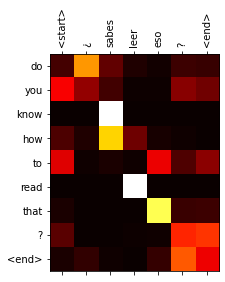
This plots the first memory attention map from the final decoder head. Try modifying it to plot maps from other locations as well as self-attention maps.
plot_attention_head(inp_sent_full.split(),
                    tar_pred_sent_full.split(),
                    attn['dec_memory'][-1][0].numpy())
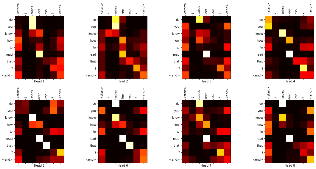
Now let us plot all the memory attention maps from the final decoder head.
def plot_attention_weights(inp_sentence, tar_sentence, attention_heads):
  fig = plt.figure(figsize=(16, 8))

  for h, head in enumerate(attention_heads):
    ax = fig.add_subplot(2, 4, h+1)

    plot_attention_head(inp_sentence, tar_sentence, head)

    ax.set_xlabel('Head {}'.format(h+1))

  plt.tight_layout()
  plt.show()
plot_attention_weights(inp_sent_full.split(),
                    tar_pred_sent_full.split(),
                    attn['dec_memory'][-1].numpy())
What’s next
There are many ways this model can be extended. We can modify the architecture or use a different dataset. Metrics like BLEU will give us a better idea of the model’s performance. At inference time we are using a simple greedy approach choosing just the best prediction at each timestep which might not necessary lead to the best overall translation. In the paper they use beam search which stores a small number of thee top predictions at each stage searches for the best overall translation among these and this typically yields better results.
This is only the tip of the iceberg with regard to what Transformers are and what they can do. Many extensions to the original architecture have been developed and there are many more applications outside of NLP (such as image recognition and image generation). I have just linked to a handful that came to mind but there are many more.
I hope to cover some of these extensions through future tutorials. In the meantime I encourage you to experiment with making your own changes to the model.