Today's learnings and re-learnings | GRU
Contents
Introduction
The Gated Recurrent Unit (GRU) comprises a state $\mathbf{h}^{(t-1)}$ and 2 “gates” a reset gate and an update gate. At each timestep the cell takes some input $x$ and uses that along with the existing value of $\mathbf{h}^{(t-1)}$ to update its state.
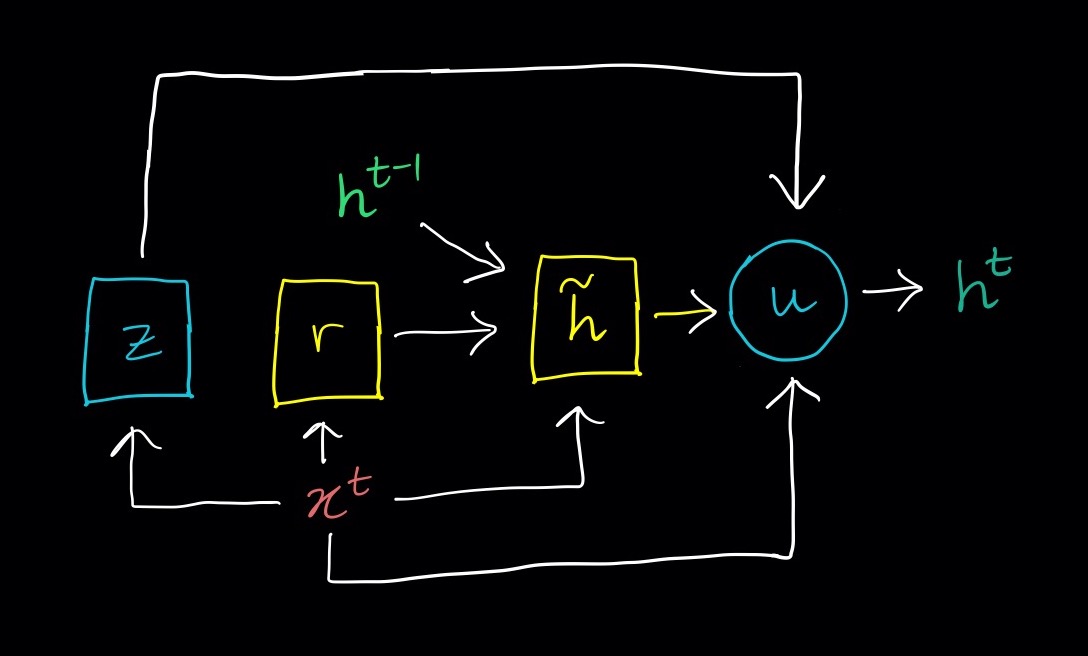
Here is a summary of what the gates do which is shown in the figure above and described in more detail below:
Reset gate (shown in blue)
- Calculate a weight $\mathbf{r}$ using $\mathbf{x}_t$ and $\mathbf{h}^{(t-1)}$.
- Propose a value for the new state $\tilde{\mathbf{h}}$ using $\mathbf{x}_t$, $\mathbf{h}^{(t-1)}$ and $\mathbf{r}$
Update gate (shown in yellow)
- Calculate a weight $\mathbf{z}$ using $\mathbf{x}_t$ and $\mathbf{h}^{(t-1)}$.
- Updates the state $\mathbf{h}^{(t)}$ using $\mathbf{x}_t$, $\mathbf{h}^{(t-1)}$, $\tilde{\mathbf{h}}$ and $\mathbf{z}$
A GRU cell is illustrated in the figure above. Steps which involve linear layers are shown as boxes in the figure whilst the final update which does not use any learned weights is shown as a circle.
Let us now delve into more details about these steps.
The equations of the GRU
Reset gate
Before it can predict the proposed new value for the state $\tilde{\mathbf{h}}^{(t)}_j$, it needs to decide how relevant each element of the previous state is likely to be for the new state. We can also think of this as predicting whether each element of the state should be reset. Again this happens via a layer with a similar format to the one used for predicting $\mathbf{z}$:
\[\tilde{\mathbf{r}}^{(t-1)} = \text{sigmoid}\left(\left(\mathbf{W}_{r}\mathbf{x}\right)_j + \left(\mathbf{U}_{r}\mathbf{h}^{(t-1)}\right)_j + \left(\mathbf{b}_{r}\right)_j\right)\]This is then multiplied element-wise with $h_{t-1}$ and the resulting vector is used along with $x$ to predict the proposed new value for the next state which is a value that varies between -1 and 1.
\[\tilde{\mathbf{h}} = \text{tanh}\left(\left(\mathbf{W}_{\tilde{h}}\mathbf{x}\right)_j + \left(\mathbf{U}_{\tilde{h}}\left(\mathbf{r} \circ \mathbf{h}^{(t-1)}\right)\right)_j + \left(\mathbf{b}_{\tilde{h}}\right)_j\right)\]where $\circ$ denotes element-wise multiplication.
Update gate
The update weight $\mathbf{z}$ which is between 0 and 1 determines how much of the previous state to keep when obtaining the next value $h_t$.
\[\tilde{\mathbf{z}} = \text{sigmoid}\left(\left(\mathbf{W}_{z}\mathbf{x}\right)_j + \left(\mathbf{U}_{z}\mathbf{h}^{(t-1)}\right)_j + \left(\mathbf{b}_{z}\right)_j\right)\]Finally we can use $z$ to obtain the value of the new state as weighted sum or equivalently a linear interpolation between the previous state and the proposed new state:
\[\mathbf{h}^{(t)}_j = \mathbf{z}_j \mathbf{h}_j^{(t-1)} + (1 - \mathbf{z}_j) \tilde{\mathbf{h}}_j^{(t)}\]The $\text{tanh}$ activation makes $\tilde{\mathbf{h}}^{(t)}$ lie between -1 and 1. The value of $\mathbf{h}^{(t)}$ must lie between $\mathbf{h}^{(t-1)}$ and $\tilde{\mathbf{h}}^{(t)}$. Since initial values of the state before the first time step, $\mathbf{h}^{(0)}_j$, are all 0 it can be seen via induction that the value of the state will be always be between -1 and 1.
The state $\mathbf{h}^{(t)}$ can then be used to make further prediction at this timestep such as an output $y_t$ or further states in case of a stacked recurrent network.
Intepretation
The update gate helps to capture long term dependencies since a higher value of $\mathbf{z}_j$ means more of the previous state is kept. In contrast the reset gate helps to capture short-term dependencies. If $\mathbf{r}_j$ is large the fraction of $\tilde{\mathbf{h}}^{(t)}_j$ used to update the state will be very little influence by the previous state. Both short and long term dependencies can be important in processing a sequence. For example in the following sentence from the paper:
In our preliminary experiments, we found that it is crucial to use this new unit with gating units.
the adjective “new” should be associated with its neighbour “unit” rather than for example with “experiments” or “units” at the end of the sentence (short-term) but to understand what it is to which “this” refers, information from earlier sentences is needed (long-term).
The idea is that elements $\mathbf{h}^{(t-1)}_j$ of the state which capture short-term dependencies will often get reset whilst others which capture long-term will be updated more slowly.