Notes on the Carnot Cycle

In this post I share some notes about the Carnot cycle with derivations of quantities for each process along with code to plot P-V and S-T diagrams for a numerical example.

Preliminaries
Carnot cycle
Process $1 \rightarrow 2$
- P-V relation
- 1st law
- 2nd law
- Summary
- Example
Process $2 \rightarrow 3$
Process $3 \rightarrow 4$
- Summary
- Example (continued)
Process $4 \rightarrow 1$
Summary
Efficiency
Summary

Preliminaries

from IPython.display import display
import numpy as np
import pandas as pd
import matplotlib.pyplot as plt
import pickle
import io

# A function to copy a matplotlib figure (adapted from https://stackoverflow.com/questions/45810557/copy-an-axes-content-and-show-it-in-a-new-figure)
def copy_fig(fig):
    buf = io.BytesIO()
    pickle.dump(fig, buf)
    buf.seek(0)
    return pickle.load(buf) 

From experimental observations of ideal gases we have the following:

P-V-T relation: $PV = mRT$ (equation of state)
If $V$ is constant during a heat transfer $Q$, the gas behaves like a solid: $Q_{12} = mc_V(T_2 - T_1)$
If the gas is subject to a constant temperature expansion / compression, we observe that $Q_{12} = W_{12}$

From which the following constitutive relations may be derived for energy and entropy

Constant volume heat transfer, from 2, $\Delta E = Q_{12} - W_{12} = Q_{12} = mc_V(T_2 - T_1)$
Since entropy change is path independent, we can split up any reversible process into two steps
- $1-1’$: constant volume
  - From observation 2, note that $\int_{1}^{1’} \delta Q = Q_{11’} = mc_V(T_{1’} - T_1 = \int_{1}^{1’} mc_V dT$
  - Which gives $S_{1’} - S_1 = \int_1^{1’}\frac{\delta Q}{T} = \int_1^{1’}mc_V\frac{dT}{T} = mc_V\ln\frac{T_{1’}}{T_1}$
- $1’-2$: constant temperature
  - From equation of state, $PV = mRT = mRT_{1’} = mRT_2 \implies P = \frac{mRT_2}{V}$
  - From observation 3, $Q_{1’2} = W_{1’2} = \int_{1’}^2 P dV = \int_{1’}^2 \frac{mRT_2}{V} dV = mRT_2\ln{\frac{V_2}{V_{1’}}}$
  - Which gives $S_2 - S_{1’} = \int_{1’}^2\frac{\delta Q}{T} = \frac{1}{T_2}\int_{1’}^\delta Q = mR\ln{\frac{V_2}{V_{1’}}}$
Combining the results whilst noting $T_{1’} = T_2$ and $V_{1’} = V_1$ you get

\[\Delta S = S_2 - S_1 = (S_2 - S_{1'}) + (S_{1'} - S_1) = mc_V\ln\frac{T_2}{T_1} + mR\ln{\frac{V_2}{V_1}}\]

From the constitutive relations for entropy and the equation of state, the following P-V relation may be derived for an isentropic process ($\Delta S = 0$):

\[PV^{\gamma} = \text{constant} \\ \gamma = \frac{c_P}{c_V} = 1 + \frac{R}{c_V}\]

Carnot cycle

Consists of four reversible processes
For each process we want to determine
- Pressure volume (P-V) relation
- Change in energy: $\Delta E$
- Heat transfer: $Q$
- Work: $W$
- Change in entropy: $\Delta S$
- The constituents of $\Delta S$:
  - Entropy transferred: $S_\text{trans}$
  - Entropy generated: $S_\text{gen}$
- Entropy temperatue (S-T) relation
Since all the processes are reversible no entropy is generated so $S_\text{gen} = 0$

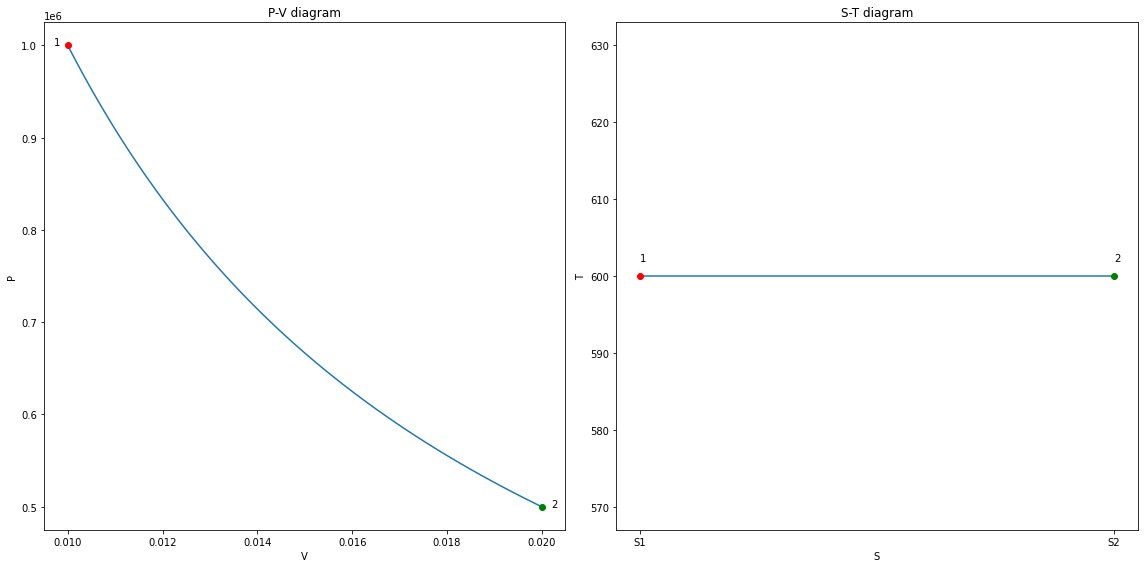
Process $1 \rightarrow 2$

Isothermal: $T_2 = T_1$
Expansion at $T_H = T_1$

P-V relation

From equation of state

\[PV = mRT = mRT_1 \implies P = \frac{mRT_1}{V}\]

1st law

Since constant temperature expansion, from observation 3: $\Delta E = 0$ $Q_{12} = W_{12} = \int_1^2 P dV = \int_1^2 \frac{mRT}{V} dV = mRT_1\ln{\frac{V_2}{V_1}}$

2nd law

Because of reversible and isothermal nature of the process, ${S_\text{gen}}$

\[\Delta S = \int_1^2 \frac{\delta Q}{T} + {S_\text{gen}}= \int_1^2\frac{\delta Q}{T} = \frac{1}{T_1}\int_1^2\delta Q = \frac{Q_{12}}{T_1} = mR\ln{\frac{V_2}{V_1}}\]

Since $S_\text{gen} = 0$

\[S_\text{trans} = \Delta S = mR\ln{\frac{V_2}{V_1}}\]

Summary

$P = \frac{mRT_1}{V}$
$\Delta E = 0$
$Q_{12} = mRT_1\ln{\frac{V_2}{V_1}}$
$W_{12} = mRT_1\ln{\frac{V_2}{V_1}}$
$\Delta S = mR\ln{\frac{V_2}{V_1}}$
- $S_\text{trans} = mR\ln{\frac{V_2}{V_1}}$
- $S_\text{gen} = 0$
On the $S-T$ diagram, since $T$ is constant, there is a straight horizontal line $T = T_1$ between $S_1$ and $S_2 = S_1 + mR\ln{\frac{V_2}{V_1}}$

Example

Some quanities for a cycle

cv = 718
R = 287
TH = 600
TC = 500
V1 = 0.01
V2 = 0.02
P1 = 1e6

We can derive other quantities from the above

T1 = TH
T2 = T1 # isothermal
# state equation to find P2 and m
m = P1 * V1 / (R * T1) 
P2 = m*R*T2/V2

print(f'm = {m}')
print(f'P2 = {P2}')

m = 0.05807200929152149
P2 = 500000.0

The P-V and S-T plots

V = np.linspace(V1, V2, 101)
P = m*R*T1 / V
assert np.isclose(P[-1], P2)
fig12, (ax1, ax2) = plt.subplots(1, 2, figsize=(16, 8))
ax1.plot(V, P)
line_clr = ax1.lines[0].get_color()
ax1.plot(V1, P1, marker='o', color='red')
ax1.plot(V2, P2, marker='o', color='green');
ax1.set_xlabel('V')
ax1.set_ylabel('P')
ax1.set_title('P-V diagram')
ax1.text(V1-3e-4, P1, '1')
ax1.text(V2 + 2e-4, P2, '2')


S1 = 1 # Some arbitrary value 
S2 = S1 + m*R*np.log(V2/V1)
ax2.plot(np.linspace(S1, S2, 101), np.ones(101)*T1)
ax2.plot(S1, T1, marker='o', color='red')
ax2.plot(S2, T2, marker='o', color='green');
ax2.text(S1, T1 + 2, '1')
ax2.text(S2, T2 + 2, '2')

ax2.set_xticks([S1, S2]);
ax2.set_xticklabels(['S1', 'S2']);
ax2.set_xlabel('S')
ax2.set_ylabel('T');
ax2.set_title('S-T diagram');

fig12.tight_layout();

png

state_df1 = pd.DataFrame(
    {'state': [1, 2],
     'P': [P1, P2],
     'V': [V1, V2],
     'T': [T1, T2]}
)

Q12 = m*R*T1*np.log(V2/V1)
W12 = Q12
dE = Q12 - W12
dS12 = S2 - S1
S_trans_12 = dS12
S_gen_12 = 0

process_df1 = pd.DataFrame(
    {'process': ['1 → 2'],
     'ΔE': [dE],
     'Q': [Q12],
     'W': [W12],
     'ΔS': [dS12],
     'S_trans': [S_trans_12],
     'S_gen': [S_gen_12]
    }
)

display(state_df1.round(5))
display(process_df1.round(5))

	state	P	V	T
0	1	1000000.0	0.01	600
1	2	500000.0	0.02	600

	process	ΔE	Q	W	ΔS	S_trans	S_gen
0	1 → 2	0.0	6931.47181	6931.47181	11.55245	11.55245	0

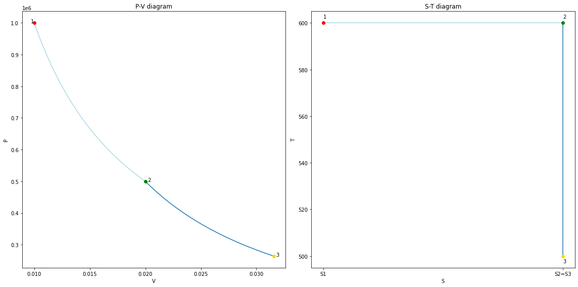
Process $2 \rightarrow 3$

Adiabatic (no heat transfer)
Expansion to $T_C = T_3 < T_2$

2nd law

Because of reversible and adiabatic nature of the process, ${S_\text{gen}}$ and $\delta Q = 0$

\[\Delta S = \int_2^3 \frac{\delta Q}{T} = 0\]

Since process is isentropic,

\[P = \frac{c}{V^{\gamma}}\]

Where $c = P_2V_2^\gamma = P_3V_3^\gamma$

1st Law

Adibatic so $Q_{23} = 0$

\[\Delta E = -W_{23} = -\int_2^3 P dV = -\int_2^3\frac{c}{V^{\gamma}} = \left.-\frac{c}{1-\gamma}V^{1-\gamma}\right\vert^{V_3}_{V_2} \\ = -\frac{1}{1-\gamma}\left(P_3V_3^\gamma V_3^{1-\gamma} - P_2V_2^\gamma V_2^{1-\gamma}\right) = -\frac{1}{1-\gamma}\left(P_3V_3 - P_2V_2\right) \\= -\frac{mR}{\frac{R}{c_V}}\left(T_3 - T_2\right) = -mc_V\left(T_3 - T_2\right)\]

Note that since $T_3 < T_2$, the energy change is positive

Summary

$P = \frac{c}{V^\gamma}$
$\Delta E = -mc_V\left(T_3 - T_2\right)$
$Q_{23} = 0$
$W_{23} = mc_V\left(T_3 - T_2\right)$
$\Delta S = 0$
- $S_\text{trans} = 0$
- $S_\text{gen} = 0$
On the $S-T$ diagram, since $S$ is constant, there is a straight vertical line at $S = S_2$ between $T_3$ and $T_2$

Example (continued)

T3 = TC
gamma = 1 + R/cv
print(f'gamma = {gamma}')
V3 = (T2/T3)**(1/(gamma-1))*V2
print(f'V3 = {V3}')
P3 = m * R * T3 / V3
print(f'P3 = {P3}')
c23 = P2*V2**gamma
print(f'c23 = {c23}')
assert np.isclose(P3, c23/V3**gamma)

gamma = 1.3997214484679665
V3 = 0.03155884186189179
P3 = 264057.00721850863
c23 = 2093.5592141183565

V = np.linspace(V2, V3, 101)
P = c23 / V**gamma
assert np.isclose(P[-1], P3)
fig23 = copy_fig(fig12)
ax1, ax2 = fig23.get_axes()
for line in ax1.lines + ax2.lines:
    if line.get_color() == line_clr:
        line.set_color('lightblue')
ax1.plot(V, P, color=line_clr, zorder=-1)
ax1.plot(V3, P3, marker='o', color='gold');
ax1.text(V3 + 2e-4, P3, '3')

S3 = S2
ax2.plot(np.ones(101)*S2, np.linspace(T2, T3, 101), color=line_clr, zorder=-1)
ax2.plot(S3, T3, marker='o', color='gold');

ax2.set_xticks([S1, S2]);
ax2.set_xticklabels(['S1', 'S2=S3']);
ax2.text(S3, T3 - 3, '3')
fig23.tight_layout();
fig23

png

state_df2 = pd.concat(
    [state_df1, 
    pd.DataFrame(
        {'state': [3],
         'P': [P3],
         'V': [V3],
         'T': [T3]}
    )], axis=0
).reset_index(drop=True)

Q23 = 0 
W23 = m*cv*(T3 - T2)
dE = Q23 - W23
dS23 = S3 - S2
S_trans_23 = dS23
S_gen_23 = 0

process_df2 = pd.concat(
    [process_df1, 
     pd.DataFrame(
    {'process': ['2 → 3'],
     'ΔE': [dE],
     'Q': [Q23],
     'W': [W23],
     'ΔS': [dS23],
     'S_trans': [S_trans_23],
     'S_gen': [S_gen_23]
    })
    ], axis=0
)

display(state_df2.round(5))
display(process_df2.round(5))

	state	P	V	T
0	1	1000000.00000	0.01000	600
1	2	500000.00000	0.02000	600
2	3	264057.00722	0.03156	500

	process	ΔE	Q	W	ΔS	S_trans	S_gen
0	1 → 2	0.00000	6931.47181	6931.47181	11.55245	11.55245	0
0	2 → 3	4169.57027	0.00000	-4169.57027	0.00000	0.00000	0

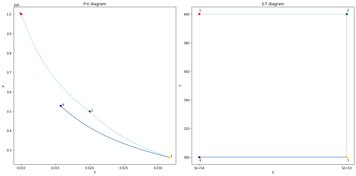
Process $3 \rightarrow 4$

Isothermal
Compression at $T_C = T_3$

The derivations are analogous to $1 \rightarrow 2$ so we can just need to replace the process ids in the results obtained earlier

Summary

$P = \frac{mRT_3}{V}$
$\Delta E = 0$
$Q_{34} = mRT_3\ln{\frac{V_4}{V_3}}$
$W_{34} = mRT_3\ln{\frac{V_4}{V_3}}$
$\Delta S = mR\ln{\frac{V_4}{V_3}}$
- $S_\text{trans} = mR\ln{\frac{V_4}{V_3}}$
- $S_\text{gen} = 0$
On the $S-T$ diagram, since $T$ is constant, there is a straight horizontal line $T = T_3$ between $S_3$ and $S_4=S_3 + mR\ln{\frac{V_4}{V_3}}$

Example (continued)

Note that to find $V_4$ we use the fact that the next process is isentropic

T4 = T3
V4 = (T1/T4)**(1/(gamma-1))*V1
P4 = m*R*T4/V4

print(f'V4 = {V4}')
print(f'P4 = {P4}')

V4 = 0.015779420930945896
P4 = 528114.0144370173

V = np.linspace(V3, V4, 101)
P = m*R*T3/V
assert np.isclose(P[-1], P4)
fig34 = copy_fig(fig23)
ax1, ax2 = fig34.get_axes()
for line in ax1.lines + ax2.lines:
    if line.get_color() == line_clr:
        line.set_color('lightblue')
ax1.plot(V, P, color=line_clr, zorder=-1)
ax1.plot(V4, P4, marker='o', color='indigo');
ax1.text(V4 + 2e-4, P4, '4')

S4 = S3 + m*R*np.log(V4/V3)
ax2.plot(np.linspace(S3, S4, 101), np.ones(101)*T3, color=line_clr, zorder=-1)
ax2.plot(S4, T4, marker='o', color='indigo');
ax2.text(S4, T4 - 3, '4')

ax2.set_xticks([S1, S2]);
ax2.set_xticklabels(['S1=S4', 'S2=S3']);
fig34.tight_layout();
fig34

png

state_df3 = pd.concat(
    [state_df2,
    pd.DataFrame(
        {'state': [4],
         'P': [P4],
         'V': [V4],
         'T': [T4]}
    )], axis=0
).reset_index(drop=True)

Q34 = m*R*T3*np.log(V4/V3)
W34 = Q34
dE = Q34 - W34
dS34 = S4 - S3
S_trans_34 = dS34
S_gen_34 = 0

process_df3 = pd.concat(
    [process_df2, 
     pd.DataFrame(
    {'process': ['3 → 4'],
     'ΔE': [dE],
     'Q': [Q34],
     'W': [W34],
     'ΔS': [dS34],
     'S_trans': [S_trans_34],
     'S_gen': [S_gen_34]
    })
    ], axis=0
)

display(state_df3.round(5))
display(process_df3.round(5))

	state	P	V	T
0	1	1000000.00000	0.01000	600
1	2	500000.00000	0.02000	600
2	3	264057.00722	0.03156	500
3	4	528114.01444	0.01578	500

process	ΔE	Q	W	ΔS	S_trans
1 → 2	0.00000	6931.47181	6931.47181	11.55245	11.55245
2 → 3	4169.57027	0.00000	-4169.57027	0.00000	0.00000
3 → 4	0.00000	-5776.22650	-5776.22650	-11.55245	-11.55245

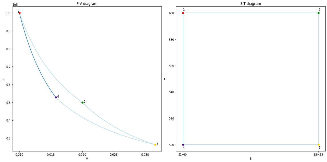
Process $4 \rightarrow 1$

Isothermal
Compression to $T_H = T_1$

The derivations are analogous to $2 \rightarrow 3$ so we can just need to replace the process ids in the results obtained earlier

Summary

$P = \frac{c}{V^\gamma}$
$\Delta E = -mc_V\left(T_1 - T_4\right)$
$Q_{41} = 0$
$W_{41} = mc_V\left(T_1 - T_4\right)$
$\Delta S = 0$
- $S_\text{trans} = 0$
- $S_\text{gen} = 0$
On the $S-T$ diagram, since $S$ is constant, there is a straight vertical line $S = S_4$ between $T_1$ and $T_4$

c41 = P4*V4**gamma
print(f'c41 = {c41}')
assert np.isclose(P1, c41/V1**gamma)

c41 = 1586.9275618720021

V = np.linspace(V4, V1, 101)
P = c41/V**gamma
assert np.isclose(P[-1], P1)
fig41 = copy_fig(fig34)
ax1, ax2 = fig41.get_axes()
for line in ax1.lines + ax2.lines:
    if line.get_color() == line_clr:
        line.set_color('lightblue')
ax1.plot(V, P, color=line_clr, zorder=-1)
ax2.plot(np.ones(101)*S4, np.linspace(T4, T1, 101), color=line_clr, zorder=-1)

fig41

png

Q41 = 0 
W41 = m*cv*(T1 - T4)
dE = Q41 - W41
dS41 = S1 - S4
S_trans_41 = dS41
S_gen_41 = 0

process_df4 = pd.concat(
    [process_df3, 
     pd.DataFrame(
    {'process': ['4 → 1'],
     'ΔE': [dE],
     'Q': [Q41],
     'W': [W41],
     'ΔS': [dS41],
     'S_trans': [S_trans_41],
     'S_gen': [S_gen_41]
    })
    ], axis=0
)

display(state_df3.round(5))
display(process_df4.round(5))

	state	P	V	T
0	1	1000000.00000	0.01000	600
1	2	500000.00000	0.02000	600
2	3	264057.00722	0.03156	500
3	4	528114.01444	0.01578	500

process	ΔE	Q	W	ΔS	S_trans
1 → 2	0.00000	6931.47181	6931.47181	11.55245	11.55245
2 → 3	4169.57027	0.00000	-4169.57027	0.00000	0.00000
3 → 4	0.00000	-5776.22650	-5776.22650	-11.55245	-11.55245
4 → 1	-4169.57027	0.00000	4169.57027	0.00000	0.00000

Efficiency

Efficiency is the following ratio $\eta = \frac{W_\text{net}}{Q_H}$

where $Q_C$ and $Q_H$ stand for the heat transferred at out of and into the system, respectively.

For a Carnot cycle

\[W_\text{net} = W_{12} + W_{23} + W_{34} + W_{41} \\ = mRT_1\ln{\frac{V_2}{V_1}} + mc_V\left(T_3 - T_2\right) + mRT_3\ln{\frac{V_4}{V_3}} + mc_V\left(T_1 - T_4\right) \\ = mRT_1\ln{\frac{V_2}{V_1}} + mc_V\left(T_3 - T_2\right) + mRT_3\ln{\frac{V_4}{V_3}} + mc_V\left(T_2 - T_3\right) \\ = mRT_1\ln{\frac{V_2}{V_1}} + mRT_3\ln{\frac{V_4}{V_3}}\]

Since

$V_3 = \left(\frac{T_2}{T_3}\right)^{\frac{1}{\gamma-1}}V_2$ $V_4 = \left(\frac{T_1}{T_4}\right)^{\frac{1}{\gamma-1}}V_1 = \left(\frac{T_2}{T_3}\right)^{\frac{1}{\gamma-1}}V_1$

we have

\[\frac{V_3}{V_4} = \frac{V_2}{V_1}\]

Hence

$W_\text{net} = mR(T_1 - T_3)\ln{\frac{V_2}{V_1}}$ $Q_C = Q_{12} = W_{12} = mRT_1\ln{\frac{V_2}{V_1}}$

which means

\[\eta = \frac{W_\text{net}}{Q_H} = 1 - \frac{T3}{T1} = 1 - \frac{T_C}{T_H}\]

Summary

fig_final = copy_fig(fig41)
ax1, ax2 = fig_final.get_axes()
for line in ax1.lines + ax2.lines:
    if line.get_color() == 'lightblue':
        line.set_color(line_clr)
display(fig_final)
display(state_df3.round(5))
display(process_df4.round(5))

png

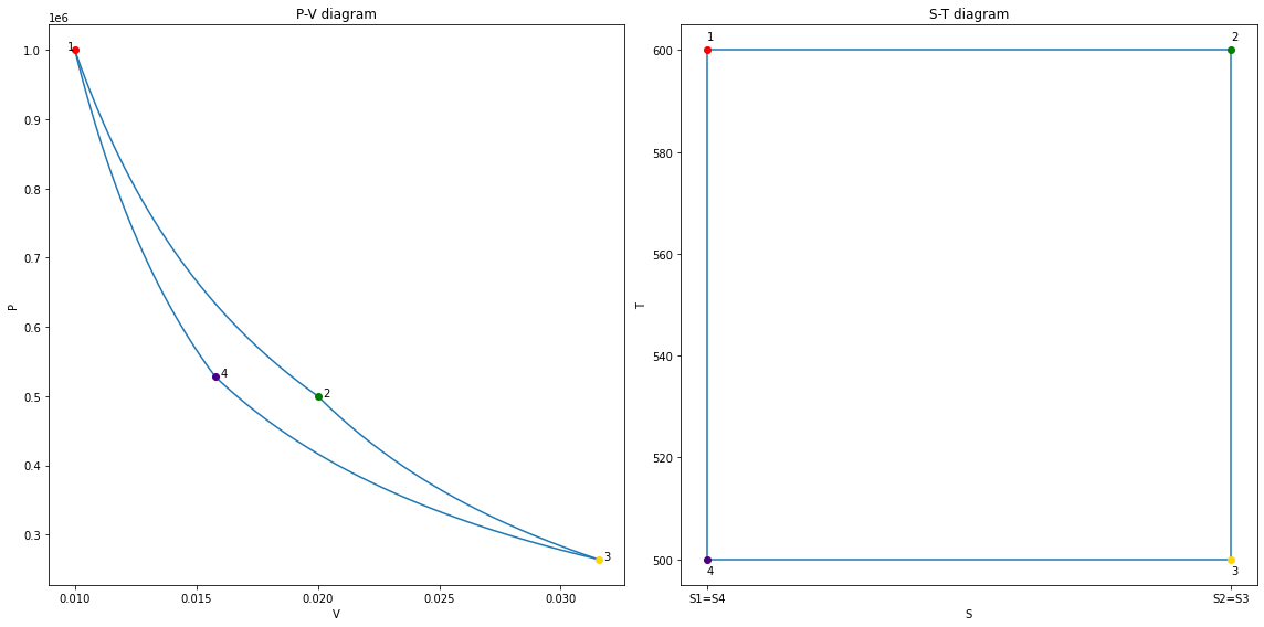
	state	P	V	T
0	1	1000000.00000	0.01000	600
1	2	500000.00000	0.02000	600
2	3	264057.00722	0.03156	500
3	4	528114.01444	0.01578	500

process	ΔE	Q	W	ΔS	S_trans
1 → 2	0.00000	6931.47181	6931.47181	11.55245	11.55245
2 → 3	4169.57027	0.00000	-4169.57027	0.00000	0.00000
3 → 4	0.00000	-5776.22650	-5776.22650	-11.55245	-11.55245
4 → 1	4169.57027	0.00000	-4169.57027	0.00000	0.00000

Contents

Preliminaries

Carnot cycle

Process $1 \rightarrow 2$

P-V relation

1st law

2nd law

Summary

Example

Process $2 \rightarrow 3$

2nd law

1st Law

Summary

Example (continued)

Process $3 \rightarrow 4$

Summary

Example (continued)

Process $4 \rightarrow 1$

Summary

Efficiency

Summary