Turbulence in Van Gogh's Artworks
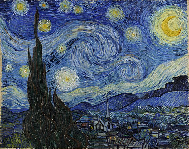
What does it mean to say that Van Gogh painted true turbulence? A paper from 2006, which makes this argument demonstrates that some of his paintings have properities that are mathematically similar to the behaviour of turbulent fluids. In this post I seek to understand these ideas by implementing some of their experiments.
Contents
- Luminance
- Probability density function
- Statistical model
- Results
- Further analysis
- Additional paintings
- AI-generated turbulence?
- Concluding remarks
Luminance
The particular property of the colours that is of interest is called luminance, which can simply be considered the pixel brightness values when converting from RGB to gray. The paper uses the following conversion formula also used by cv2 for grayscale conversion
where $r, g, b$ are the colours.
It is suggested that the luminance differences at different length scales in some of the artworks by Vincent Van Gogh follow a distribution characteristic of turbulence.
import cv2
from PIL import Image
import numpy as np
import tqdm.autonotebook as tqdm
import matplotlib.pyplot as plt
import pandas as pd


NUM_CLRS = 255
CLR_RANGE= np.arange(-NUM_CLRS, NUM_CLRS+1)
CLRS = CLR_RANGE.astype('float')
Probability density function
The paper does not go into details of how the luminance differences are calculated. I have arbitrarily implemented the method as follows for an image of dimensions $h \times w$
- For each pixel location $i, j$ and length-scale $a$, traverse the rows from $i-a$ to $i + a$
- For each row $i’$, find column indices $j’_{\pm} = \text{round}\left(j \pm \left(a^2 - (i’ - i)^2 \right)^\frac{1}{2} \right)$
- If $i’< 0$ or $i’ > h-1$ or $j’_{\pm}< 0$ or $j’_{\pm} > w-1$ then relevant pixel is out of bounds so skip
- Find $du_{i’j’_\pm ij} = u_{i’j’_\pm} - u_{ij}$
def lum_densities(arr, dist, indices=None, batch_size=None, bar=False):
    """
    Calculates luminance differences across pixels in `arr` that are approximately `dist` apart
    """

    counts = np.zeros(len(CLR_RANGE), dtype='int')

    # Calculate for selected pixels only (for batchwise calculation)
    if indices is None:
        rows, colms = np.stack(np.indices(arr.shape[:2]), -1).reshape((-1, 2)).T
    else:
        rows, colms = indices

    if batch_size is not None:
        print('Using batches')
        n_batches = int(np.ceil(len(rows) / batch_size))
        iterable = tqdm.trange(n_batches) if bar else range(n_batches)

        for i in iterable:
            slc = slice(i*batch_size, (i+1)*batch_size)
            counts += lum_densities(arr, dist, indices=(rows[slc], colms[slc]))

        return counts

    row_range = np.arange(-dist, dist + 1)
    idx_row0 = rows[:, None] + row_range
    dist_colm = np.sqrt(dist**2 - row_range**2)
    dist_colm = np.concatenate([dist_colm, -dist_colm[..., 1:-1]], -1)
    idx_colm0 = colms[:, None] + dist_colm

    idx_row = np.concatenate([idx_row0, idx_row0[..., 1:-1]], -1)

    idx_colm = np.round(idx_colm0)

    cond_row = np.logical_and(idx_row >= 0, idx_row <arr.shape[0])
    cond_colm = np.logical_and(idx_colm >= 0, idx_colm <arr.shape[1])

    cond = np.logical_and(cond_row, cond_colm)

    idx_row2 = idx_row[cond]
    idx_colm2 = idx_colm[cond]

    rows2 = np.tile(rows[:, None], idx_row.shape[-1])[cond]
    colms2 = np.tile(colms[:, None], idx_colm.shape[-1])[cond]

    # convert to int to ensure negative differences can be found
    lum_vals = cv2.cvtColor(arr, cv2.COLOR_RGB2GRAY).astype('int')

    du = lum_vals[idx_row2, idx_colm2.astype('int')] - lum_vals[rows2, colms2]

    # Instead of np.unique as we don't need to sort so faster
    val_counts = pd.value_counts(du, sort=False)

    # num = -255,...,255 -> 0,...,510
    idx = NUM_CLRS + val_counts.index.values
    counts[idx] = val_counts.values

    return counts

    #return du
A function to faciliate calculating densities and moments in batched fashion for large length scales.
def find_densities(arr, dists,  batch_limit=None, batch_size=10000, bar=True,
                   batch_bar=True, return_moments=False,
                  moment_nums=(1, 2, 3, 4, 5, 6, 7, 8, 9)):

    n_dists = len(dists)
    dens_norm = np.zeros((n_dists, len(CLR_RANGE)))
    dens_orig = np.zeros_like(dens_norm)
    stds = np.zeros(n_dists)
    if return_moments:
        moments = np.zeros((n_dists, len(moment_nums)))

    iterable = enumerate(dists)
    if bar:
        iterable = tqdm.tqdm(iterable, total=len(dists))
    batching = False

    for i,dist in iterable:
        if not batching and batch_limit is not None and dist > batch_limit:
            print('Batching starting')
            batching = True
        den = lum_densities(arr, dist, batch_size=None if not batching else batch_size, bar=batch_bar)
        den = den.astype('float')
        # Normalise by area under curve
        area = ( (CLRS[1:] - CLRS[:-1]) * (den[1:] + den[:-1]) / 2.).sum()
        den /= area

        assert np.isclose(den.sum(), 1)

        # Assume mean ~ 0
        std = (CLRS ** 2 * den).sum() ** .5

        du_abs = np.abs(CLRS)

        if return_moments:
            for idx, n in enumerate(moment_nums):
                moments[i, idx] = (du_abs ** n * den).sum()


        den_norm = den * std

        dens_norm[i] = den_norm
        dens_orig[i] = den
        stds[i] = std


    return (dens_norm, dens_orig, stds) + ((moments,) if return_moments else ())
    #return lum_dict, lum_orig
The paper presents plots of histograms for several artworks by Van Gogh based on images of different dimensions. They state that to rule out scaling artifacts they recalculate the luminance probability densities for images with lower resolutions and find that there are no significant differences down to fairly small resolutions (150×117 pixels) at which scale the brushwork details are lost.
Therefore, in the interests of speed I used comparatively small images, adjusting the length scales $a$ accordingly.
artworks = [
    "Starry Night",
    "Road with Cypress and Star",
    "Wheat Field with Crows",
    "Self-portrait with pipe and bandaged ear",
]

densities = {}
densities_orig = {}
stds = {}
imgs = {}
distances = [2, 5, 15, 20, 30, 60]

for artwork in artworks:
    img = imgs[artwork] = Image.open(f'van_gogh_art/{artwork.replace(" ", "_")}.jpeg')
    arr = np.array(img)
    densities[artwork], densities_orig[artwork], stds[artwork] = find_densities(arr, distances, batch_limit=10, batch_bar=True)
Statistical model
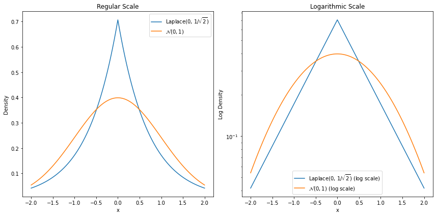
When the luminance differences have been found, the log probability density function (PDF) at each scale can be approximated. If the distributions go from roughly a Laplacian distribution at small length scales to a normal distribution at larger length scales, it suggests that there is turbulence. In regular and log-normal form, these two distributions look as follows
According to the model adopted in the paper, the PDF is considered to be the weighted sum of Gaussian distributions at different scales. The paper does not give details of the model so I relied on the description from another paper which uses the same model. The paper gives the following expression for the PDF, where $d\psi$ denotes the change in the quantity of interest, here the luminance:
\[P\left(d\psi\right) = \int P\left(d\psi, \sigma\right) G\left(\sigma\right)d\sigma\]where $P\left(d\psi, \sigma\right)$ is a Gaussian with variance $\sigma^2$ and $G$ is a log-normal distribution of $\sigma$:
\[G\left(\sigma\right)= \frac{1}{\sigma\lambda \sqrt{2\pi}}\exp\left[-\frac{\ln^2\left(\sigma/\sigma_0\right)}{2\lambda^2}\right]\]For small $\lambda$, $G$ behaves like delta function around $\sigma_0$, $\delta(\sigma - \sigma_0)$ and the integral reduces to $P\left(d\psi, \sigma_0\right)$ which is a Gaussian with variance $\sigma_0^2$
The integral becomes
\[P\left(d\psi\right) = \int P\left(d\psi, \sigma\right) G\left(\sigma\right)d\sigma \\= \int\left(\frac{1}{\sigma \sqrt{2\pi}} \exp\left[{-\frac{d\psi^2}{2\sigma^2}}\right]\right)\left(\frac{1}{\sigma\lambda \sqrt{2\pi}}\exp\left[-\frac{\ln^2\left(\sigma/\sigma_0\right)}{2\lambda^2}\right] d\sigma\right) \\ = \int\frac{1}{\lambda \sigma^2 2\pi}\exp\left[{-\frac{d\psi^2}{2\sigma^2}}\right]\exp\left[-\frac{\ln^2\left(\sigma/\sigma_0\right)}{2\lambda^2}\right]d\sigma\]The goal is to estimate $P\left(d\psi\right)$ from the images and then try to fit the model to this data. My approach was as follows:
- Start with some initial values of $\sigma_0$ and $\lambda$
- Approximate the integral numerically between 0 and infinity for each value of $du$
- Use some optimisation method to update the values of $\sigma_0$ and $\lambda$
I optimised the parameters in log space and fitted them to minimise cross-entropy loss between the $P(d\psi)$ and the estimated density. My approached yielded $\lambda$ values that behaved as expected, decreasing with increasing length scale in the presence of turbulence but they are different from the range of values reported in the paper but I use smaller images and different length scales.
import scipy.integrate as integrate
import scipy.optimize as optimize

# Define the integrand function
def integrand(sigma, du, log_sigma_0, log_lambda_):
    lambda_ = np.exp(log_lambda_)
    sigma_0 = np.exp(log_sigma_0)
    term1 = 1 / (lambda_ * sigma**2 * 2 * np.pi)
    term2 = np.exp(-du**2 / (2 * sigma**2))
    term3 = np.exp(-np.log(sigma / sigma_0)**2 / (2 * lambda_**2))
    return term1 * term2 * term3

# Define the function to perform the numerical integration
def integrate_expression(du, log_sigma_0, log_lambda_, lims=(0, float('inf'))):
    result, _ = integrate.quad(integrand, *lims, args=(du, log_sigma_0, log_lambda_))
    return result

# Define the objective function to minimize
def objective(params, du_values, observed_values, lims=(0, float('inf'))):
    log_sigma_0, log_lambda_ = params
    integrated_values = np.array([integrate_expression(du, log_sigma_0, log_lambda_, lims=lims) for du in du_values])
    bin_width = du_values[1]-du_values[0]
    # -E_p(x)[log(q(x))] ~ -sum_xi p(xi) * log(q(xi)) * dx_i
    return -(observed_values * np.log(integrated_values) * bin_width).sum()


# Initial guesses for sigma_0 and lambda
initial_log_sigma_0 = 0.
initial_log_lambda = 0.
def callback(params):
    print(f"Current params: log_sigma_0 = {params[0]}, log_lambda = {params[1]}")


def fit_function(initial_log_sigma_0, initial_log_lambda, du_values, observed_values, lims=(0, float('inf'))):
    # Perform the optimization
    result = optimize.minimize(objective,
                               [initial_log_sigma_0, initial_log_lambda],
                               args=(du_values, observed_values, lims),)

    # Optimal parameters
    return result
vals = {}
for artwork in artworks:
    print(f'Finding parameters for {artwork}')
    vals[artwork] = {}
    for dist_val, den, std in zip(distances, densities[artwork], stds[artwork]):
        b = fit_function(initial_log_sigma_0, initial_log_lambda, CLRS/std, den)
        optimal_sigma_0, optimal_lambda = list(map(np.exp, b.x))
        print(f'\tDistance: {dist_val}, 𝜆 = {optimal_lambda:.4f}, 𝜎0 = {optimal_sigma_0:.4f}, loss: {b.fun:.5f}')
        vals[artwork][dist_val] = b

    print('\n\n')
Finding parameters for Starry Night
	Distance: 2, 𝜆 = 0.4760, 𝜎0 = 0.8133, loss: 1.36947
	Distance: 5, 𝜆 = 0.3739, 𝜎0 = 0.8787, loss: 1.39698
	Distance: 15, 𝜆 = 0.2951, 𝜎0 = 0.9217, loss: 1.40963
	Distance: 20, 𝜆 = 0.2642, 𝜎0 = 0.9363, loss: 1.41274
	Distance: 30, 𝜆 = 0.2083, 𝜎0 = 0.9593, loss: 1.41636
	Distance: 60, 𝜆 = 0.0500, 𝜎0 = 0.9975, loss: 1.41893


Finding parameters for Road with Cypress and Star
	Distance: 2, 𝜆 = 0.3979, 𝜎0 = 0.8678, loss: 1.39581
	Distance: 5, 𝜆 = 0.2839, 𝜎0 = 0.9275, loss: 1.41121
	Distance: 15, 𝜆 = 0.2112, 𝜎0 = 0.9582, loss: 1.41622
	Distance: 20, 𝜆 = 0.1845, 𝜎0 = 0.9677, loss: 1.41727
	Distance: 30, 𝜆 = 0.1367, 𝜎0 = 0.9819, loss: 1.41838
	Distance: 60, 𝜆 = 0.0018, 𝜎0 = 1.0000, loss: 1.41894


Finding parameters for Wheat Field with Crows
	Distance: 2, 𝜆 = 0.5367, 𝜎0 = 0.7682, loss: 1.34357
	Distance: 5, 𝜆 = 0.4553, 𝜎0 = 0.8251, loss: 1.37357
	Distance: 15, 𝜆 = 0.3708, 𝜎0 = 0.8790, loss: 1.39591
	Distance: 20, 𝜆 = 0.3471, 𝜎0 = 0.8927, loss: 1.40044
	Distance: 30, 𝜆 = 0.3091, 𝜎0 = 0.9133, loss: 1.40646
	Distance: 60, 𝜆 = 0.2285, 𝜎0 = 0.9510, loss: 1.41483


Finding parameters for Self-portrait with pipe and bandaged ear
	Distance: 2, 𝜆 = 0.7253, 𝜎0 = 0.6172, loss: 1.22429
	Distance: 5, 𝜆 = 0.7517, 𝜎0 = 0.6213, loss: 1.24452
	Distance: 15, 𝜆 = 0.7546, 𝜎0 = 0.6377, loss: 1.27172
	Distance: 20, 𝜆 = 0.7478, 𝜎0 = 0.6461, loss: 1.28114
	Distance: 30, 𝜆 = 0.7336, 𝜎0 = 0.6611, loss: 1.29654
	Distance: 60, 𝜆 = 0.6223, 𝜎0 = 0.7535, loss: 1.36785
def make_plot(img_name, imgs, distances, densities, stds, vals=None, axes=None):
img = imgs[img_name]
densities = densities[img_name]
stds = stds[img_name]
w, h = img.size
if axes is None:
_, axes = plt.subplots(1, 2, figsize=(16, 6 ))
(ax1, ax2) = axes
ax1.imshow(img)
ax1.axis('off')
for i, (dist, den, std) in enumerate(zip(distances, densities, stds)):
diff = np.exp(i*2)
label = f'{dist}'
du_norm = CLR_RANGE / std
if vals is not None:
mask = np.abs(du_norm) <= 5
optimal_log_sigma_0, optimal_log_lambda = vals[img_name][dist].x
est = np.array([integrate_expression(du, optimal_log_sigma_0, optimal_log_lambda) for du in du_norm])
lam = np.exp(optimal_log_lambda)
label += f' ($\\lambda$={lam:.4f})'
ax2.semilogy(du_norm[mask], est[mask] *diff, color='k')
ax2.semilogy(du_norm, den*diff, marker='.', markersize=8, linewidth=0, label=label, alpha=0.2)
ax2.legend();
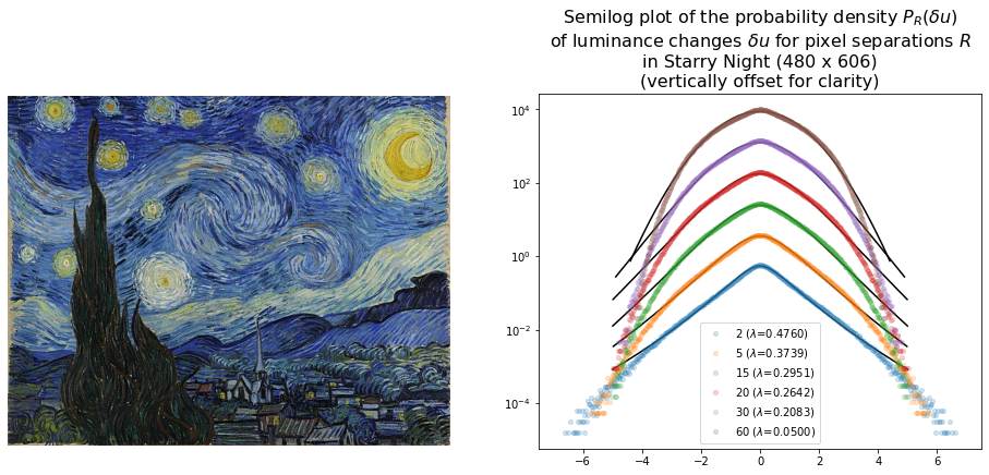
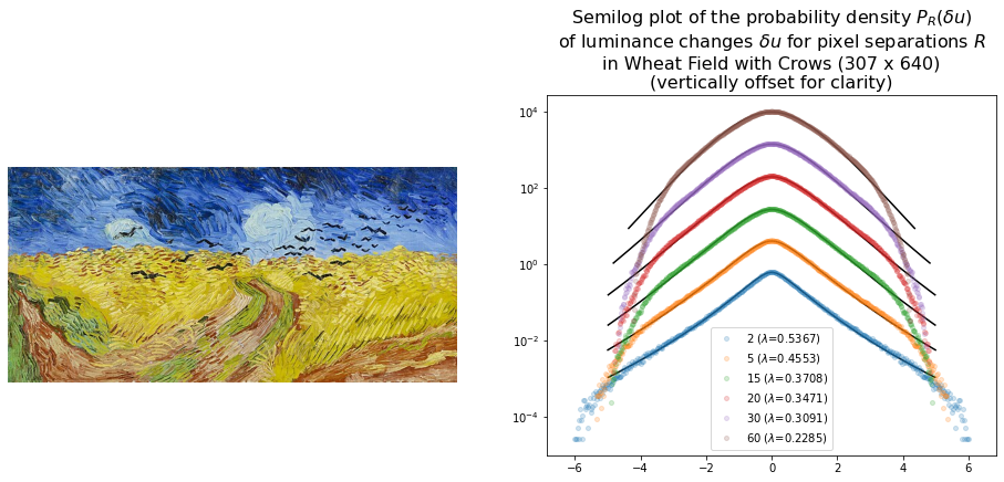
ax2.set_title('Semilog plot of the probability density $P_R(\\delta u)$\nof luminance changes $\\delta u$ for pixel separations $R$\n'
+f'in {img_name} ({h} x {w})\n(vertically offset for clarity)', fontsize=16)
Results
The densities for Starry Night seem to follow a pattern consistent with turbulence as can be seen from the plot below. The $\lambda$ values also decrease with increasing length scale and visually the model fits the data well up to a wide range of values.
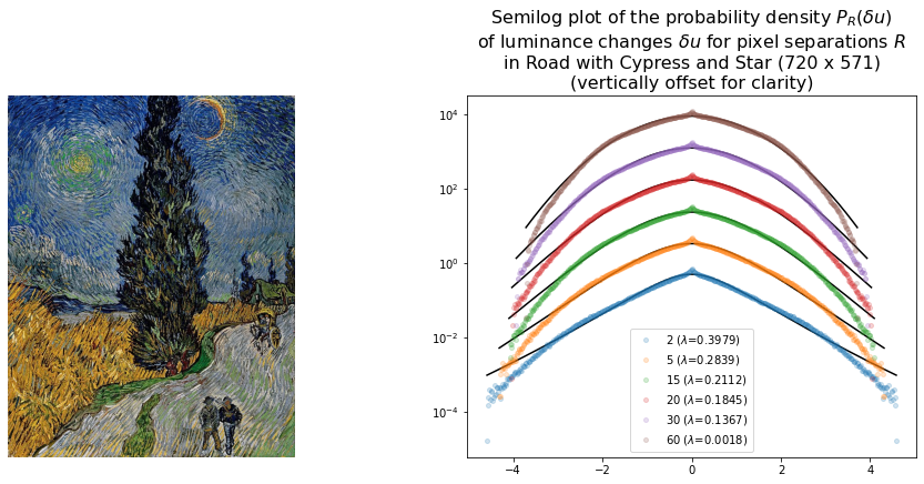
The distribution of luminance changes in Wheat Field with Crows and Road with Cypress and Star also have forms suggestive of turbulence.
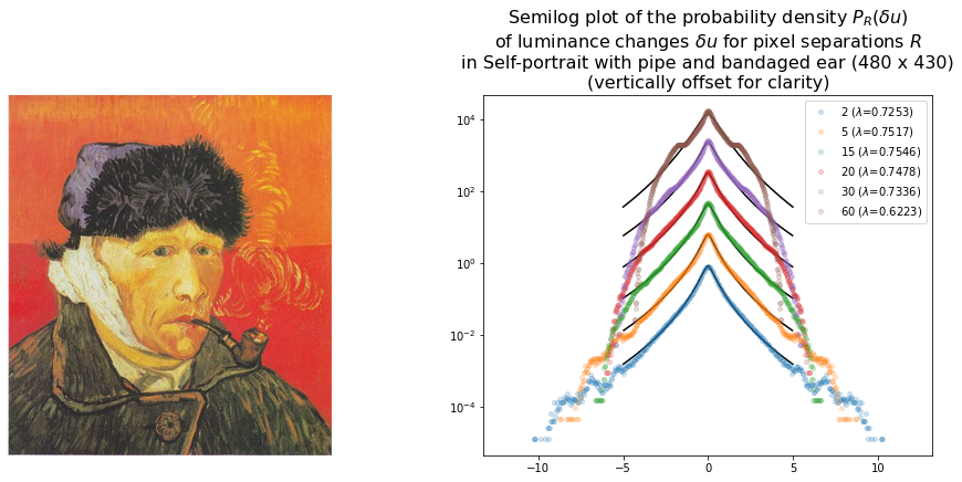
However the density plot for Self-portrait with pipe and bandaged ear departs from the expected form for turbulent behaviour. This can be seen from the shape of the plot as well as the fact lambda values fail to decrease with increasing length scales in a consistent fashion.
Further analysis
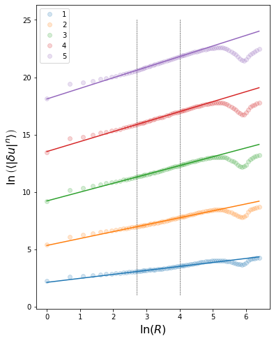
Kolmogorov hypothesised that $\left< du_R^n \right> \propto R^{\xi_n}$. In logspace this means
\[\ln\left(\left< du_R^n \right > \right) = \xi_n\ln R + Z\]where $Z$ is some intercept.
To determine if this holds for Starry Night, we calculate moments for several values of $n$ for a range of length scales.
distance_values = np.unique(
    np.concatenate(
        [distances, np.logspace(0, np.log10(600), 100).astype('int')]
    )
)
moment_nums = list(range(1, 10))
pbar = tqdm.tqdm(distance_values[::-1])
data = {}
for dval in pbar:
    pbar.set_description_str(f'dist={dval}')
    data[dval] = find_densities(arr, [dval],
                                batch_limit=10,
                                bar=False,
                                batch_bar=True,
                                batch_size=1000,
                                return_moments=True,
                                moment_nums=moment_nums)
moments = {n: np.stack([data[dval][-1].squeeze()[idx] for dval in distance_values])
           for idx, n in enumerate(moment_nums)}
Finding and plotting the first 5 moments ($n = 1, 2, 3, 4, 5$) against the length scale in a log-log plot, we can see that there seems to be a linear relationship between $R$ and the moments in log space. The plots are fit with a straight line using least squares, restricting the data to the region between the dashed lines where the plot is noticeably linear.
lst_vals = {}
plt.figure(figsize=(6, 8))
xmin, xmax = [2.7, 4.]
for n in np.arange(1,6):
    a = np.log(distance_values)
    b = np.log(moments[n]) #


    mask = np.logical_and(a>=xmin, a <=xmax)
    A = np.vstack([a, np.ones(len(a))]).T
    # Perform least squares fitting
    params, residuals, rank, s = np.linalg.lstsq(A[mask], b[mask], rcond=None)

    # Extract the slope and intercept
    slope, intercept = params
    lst_vals[n] = params
    l = plt.plot(a, A @ params)
    plt.plot(a, b,
        label = n, marker='o', linewidth=0,
                  color=l[-1].get_color(),
             alpha=0.2
    )

ymin, ymax = plt.ylim()
plt.vlines(ymin=ymin, ymax=ymax, x=[xmin,xmax], zorder=-100, linestyle='--', linewidth=0.5, color='k')
plt.xlabel('$\\ln(R)$', fontsize=16)
plt.ylabel('$\\ln\\left(\\left<\\left|\\delta u\\right|^n \\right>\\right)$', fontsize=16)
plt.legend();
Kolgomorov further hypothesised that $\xi_n$ linearly depends on $n$, in particularl that $\xi_n = n/3$. However due to the intermittent nature of turbulence there will be deviations from this model.
We use a local least-squares method found in this [paper] to estimate $\xi_n$
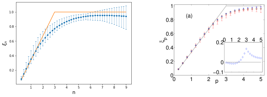
This was the part where I was not able to recreate a similar plot to the paper. Theirs shows a linear dependance of $\xi_n$ on $n$ albeit not $n/3$ up to large values of $n$ although with larger errors as $n$ increases, which is consistent with the idea of deviation from the linear model at large values of $n$, where it follows a concave curve below the $n/3$ line.
It is possible that some scaling issues are involved either in the distances or moments which is responsible for this behaviour.
However the plot is similar to the one in the paper containing the method, staying close to $n/3$ for $n < 3$ then going towards 1 then starting to move away.
a = np.log(distance_values)
mask = np.logical_and(a>=xmin, a<=xmax)
a_inner = a[mask]

slopes = {}
nvals = moment_nums

for n in nvals:

    b = np.log(moments[n])
    b_inner = b[mask]

    slopes[n] = []

    for i in range(len(a_inner)-3 + 1):
        _A = np.vstack([a_inner[i:3+i], np.ones(3)]).T
        # Perform least squares fitting
        params, residuals, rank, s = np.linalg.lstsq(_A, b_inner[i:3+i], rcond=None)

        slope, intercept = params
        slopes[n].append(slope)


    slopes[n] = np.stack(slopes[n])


slope_means = np.stack([slopes[n].mean() for n in nvals])
plt.figure()
plt.errorbar(nvals,
             slope_means,
             yerr=[slope_means-[slopes[n].min() for n in nvals],
                   [slopes[n].max() for n in nvals]-slope_means],
             fmt='o-', capsize=5);

plt.xlabel('n', fontsize=16)
plt.ylabel('$\\xi_n$', fontsize=16);
plt.plot(nvals, np.minimum(np.stack(nvals)/3, 1));
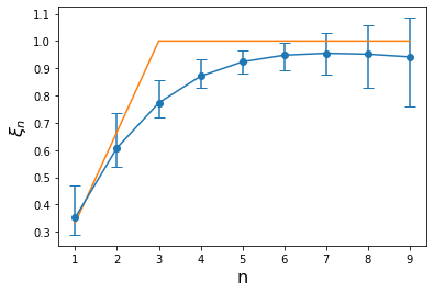
The pattern can be seen better by using more values of $n$, with the plot from the paper shown on the right.
Finally $\lambda^2$ seems to decrease linearly with $ln(R)$, which is also consistent with the paper’s findings.
b = np.stack([np.exp(vals['Starry Night'][dval].x[-1])**2 for dval in distances])
A = np.vstack([ np.log(distances), np.ones(len(distances))]).T
params, residuals, rank, s = np.linalg.lstsq(A, b, rcond=None)
plt.figure(figsize=(6, 4))
# Extract the slope and intercept
slope, intercept = params
lst_vals[n] = params
l = plt.semilogx(distances, A @ params)
plt.semilogx(distances, b,
    label = n, marker='o', linewidth=0,
              color=l[-1].get_color(),
         alpha=0.8
)
plt.xlabel('$\\ln(R)$', fontsize=16)
plt.ylabel('$\\lambda^2$', fontsize=16);

Additional paintings
For further comparison here are some plots for couple artworks by other artists which may also be considered to have a turbulent quality:
- Snow Storm - Steam-Boat off a Harbour’s Mouth by JMW Turner
- The Scream by Edvard Munch
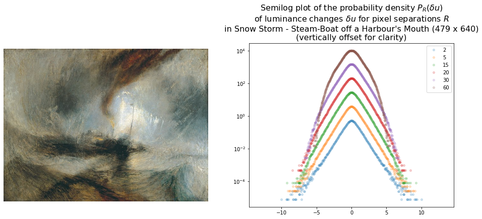
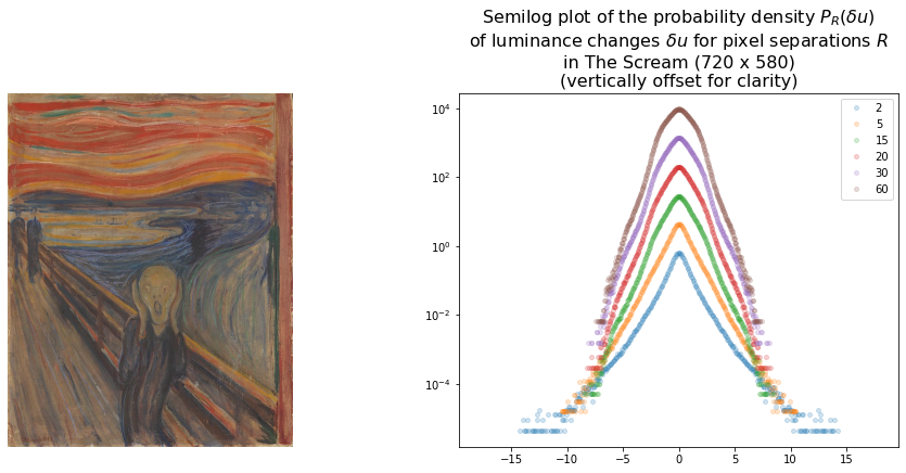
Turner’s painting yields a result that is more suggestive of turbulence than The Scream although not overwhelmingly so.
AI-generated turbulence?
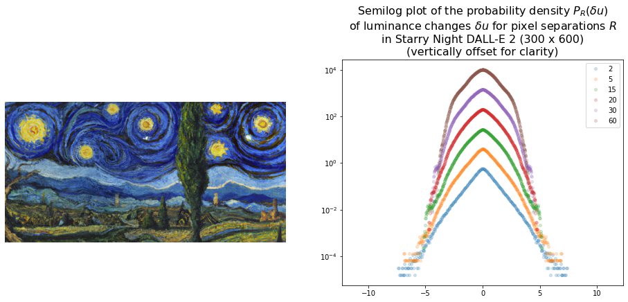
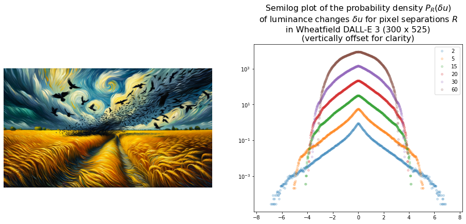
Finally here are some plots for AI-generated Van Gogh style images.
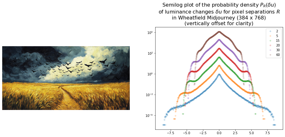
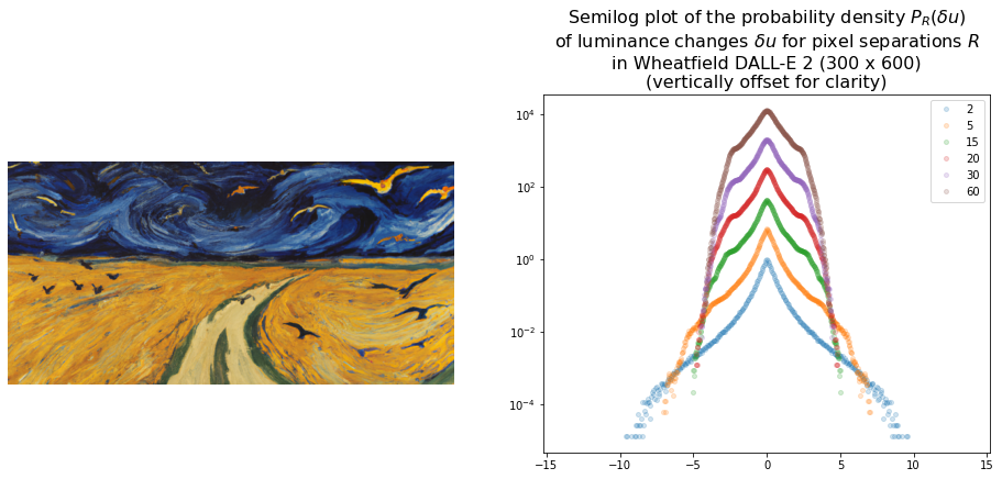
The prompt for Wheatfield with Crows was
A dramatic, cloudy sky filled with crows over a bright yellow wheat field in the style of Van Gogh. A sense of isolation is heightened by a central path leading nowhere and by the uncertain direction of flight of the crows. The windswept wheat field fills two-thirds of the canvas. oil on canvas, acclaimed, masterpiece
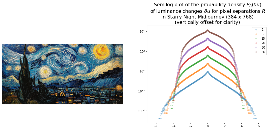
For Starry Night it was
Starry Night, an oil on canvas in the style of Vincent van Gogh. The sky features swirling brushstrokes of bright blue and white stars. There is a small village below, adding depth to the composition and a large cypress tree on the left side. The painting features detailed brushwork that captures the night’s darkness while also showcasing the light emanating from distant stars. The color palette includes shades of blue. The sky is full of swirling stars and a glowing yellow moon on the right illuminating a small village below.
All images were resized to be of a similar scale to the other images.
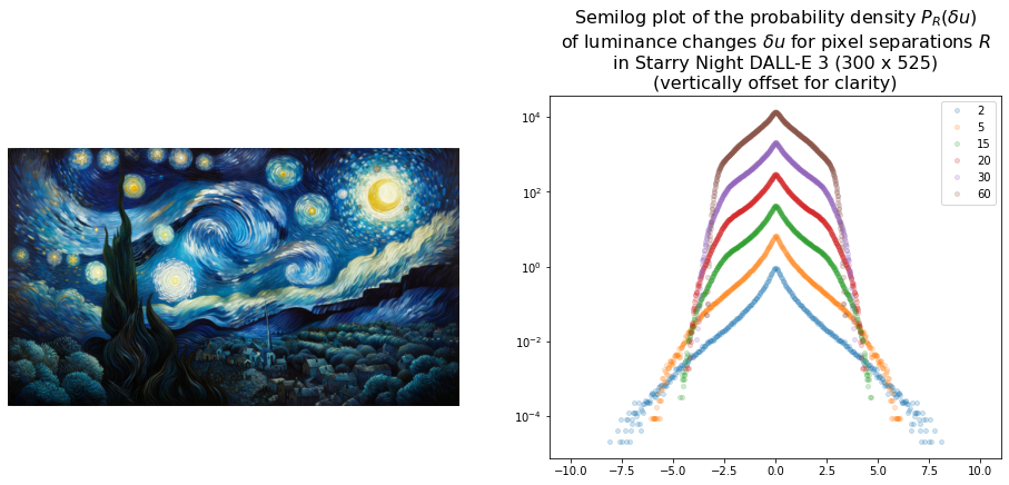
The DALL-E 2 images were generated by first generating a variation of a central crop of the original work which was then outpainted using the prompts. Since the other two models are more powerful they did not get the image as an input. Nevertheless both DALL-E-3 and Midjourney seem to produce images overly similar to the original in case of Starry Night. However neither exhibit PDFs consistent with Starry Night which suggests that it isn’t only the swirling regions that matter but the luminance must also vary in a turbulent fashion.
Interestingly the only artwork that does have a PDF suggestive of turbulence is DALL-E 3’s Wheatfield which notably has a sky that somewhat resembles Starry Night.
It’s an area worth investigating further.
Concluding remarks
This post is a preliminary exploration and may contain some inaccuracies, particularly in scaling or model interpretation. Despite this, the figures indicate turbulence in several of the artworks. My goal was to write up these initial notes in a one location, and I hope to revisit and refine the ideas further, addressing any issues along the way. In particular I would like to
- Experiment with different sizes of artwork
- Try out different length scales - I just copied one set of length scales from the paper which yields satisfactory results but a more careful choice might lead to better insights
- Understand the underlying concepts and models in more depth