TIL - B-Spline
Definition
A b-spline is a piecewise polynomial of order $p$ defined with respect to
- $m+1$ knots $t_0, \cdots, t_m$
- $n+1$ control points $a_0, \cdots, a_n$
where $p = m - n - 1$
First you generate $n+1$ polynomials $N_{i, p}(t)$ in the following recursive fashion
\[\begin{align*} N_{i, 0}(t) = \left\{ \begin {aligned} & 1 \quad & t_i \leq t < t_{i+1}, t_i < t_{i+1} \\ & 0 \quad & \text{else} \end{aligned} \right. \end{align*}\] \[N_{i, j}(t) = \frac{t - t_i}{t_{i + j} - t_i}N_{i-1, j-1}(t) + \frac{t_{i + j + 1} - t}{t_{i + j + 1} - t_{i + 1}}N_{i+1, j-1}(t), \quad j=1,2,\ldots, p\]The B-spline curve of order $p$ is the weighted sum of the control points and the curves $N_{i,p}(t)$
\[C_p(t) = \sum_{i=0}^{n} a_i N_{i,p}(t)\]Implementation
import numpy as np
import matplotlib.pyplot as plt
import sympy as sy
def bspline(t, i, p, knots):
    ti = knots[i]
    ti_p1 = knots[i+1]

    if p == 0:

        cond= sy.And(
            t >= ti,
            t < ti_p1,
            ti < ti_p1
        )

        return sy.Piecewise((sy.Number(1), cond), (sy.Number(0), True))

    ti_pp = knots[i+p]
    ti_pp1 = knots[i+p+1]

    spline1 = bspline(t, i, p-1, knots)
    spline2 = bspline(t, i + 1, p-1, knots)

    res = sy.Number(0)
    if not np.isclose(ti_pp - ti, 0):
        res += (t - ti) / (ti_pp - ti) * spline1
    if not np.isclose(ti_pp1 - ti_p1, 0):
        res +=(ti_pp1 - t) / (ti_pp1 - ti_p1) * spline2

    return res


def bspline_curve(
    t,
    knots,
    controls
):
    curve = 0
    m = len(knots) - 1
    n = len(controls) - 1
    p = m - n - 1
    for i in range(n + 1):
        curve += controls[i] * bspline(t, i, p, knots)

    return curve
Validity of indices
If bspline is initially called with $0 \leq i_\text{init} \leq n$, $p_\text{init} = m - n - 1$, then the index into knots is always within bounds i.e. $0 \leq \text{idx} \leq m$ since:
- At each step $p$ goes down by 1
- At each step $i$ goes up by a maximum of 1
Hence $i + p \leq i_\text{init} + p_\text{init}$.
Since the indices into knots are $i, i+1, i+p, i+p+1$, $\text{idx}$ and
- $i$ starts off non-negative and is non-decreasing (going up by 1 or 0) so $i \geq 0$ always
- There are at most $p_\text{init}$ such steps since the recursion ends when $p=0$ so $p \geq 0$ always
$\text{idx} \geq 0$ always.
Since largest index into knots is
\[i + p + 1 = i_\text{init} + p_\text{init} + 1 \leq n + p_\text{init} + 1 = n + m - n - 1 + 1 = m\]$\text{idx} \leq m$ always.
(Note the above includes the case when $p=0$ when the largest index $i + 1 = i + 0 + 1 = i + p + 1$).
Examples
def plot_bspline_curve_examples(
    knots,
    controls,
    colors=None,
    derivatives=(),
):
    vals = np.linspace(np.min(knots), np.max(knots), 101)
    tsy = sy.Symbol('t', real=True)
    curve = bspline_curve(
            t=tsy,
            knots=knots,
            controls=controls
        ).simplify().collect(tsy)

    def _clr(idx):
        return dict(color=colors[idx]) if colors is not None else dict()
    plt.figure(figsize=(12, 8))
    plt.plot(vals, sy.lambdify(tsy, curve)(vals), **_clr(0))

    for idx, order in enumerate(derivatives, 1):
        plt.plot(vals, sy.lambdify(tsy, curve.diff(tsy, order))(vals), **_clr(idx), label=order)

    derv_str =  (f' with derivative{"s" if len(derivatives) > 1 else ""} of order {",".join(map(str, sorted(derivatives)))},'
                 if len(derivatives) > 0 else ',')

    plt.title(f'B-spline of order {len(knots) - len(controls) - 1}{derv_str}\nknots {knots},\ncontrols {controls}')
    if len(derivatives) > 0:
        plt.legend();
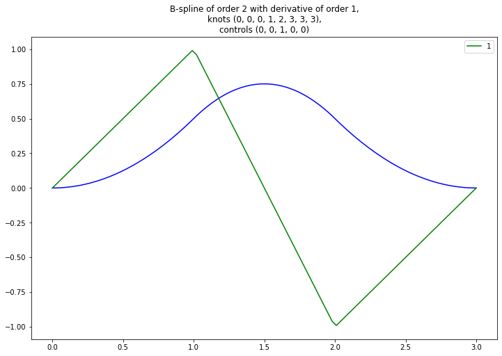
plot_bspline_curve_examples(
    knots=(0, 0, 0, 1, 2, 3, 3, 3),
    controls=(0, 0, 1, 0, 0),
    colors=['blue', 'green'],
    derivatives=[1]
)
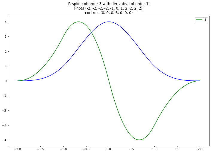
plot_bspline_curve_examples(
    knots=(-2, -2, -2, -2, -1, 0, 1, 2, 2, 2, 2),
    controls=(0, 0, 0, 6, 0, 0, 0),
    colors=['blue', 'green'],
    derivatives=[1]
)
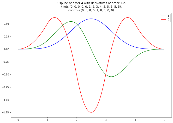
plot_bspline_curve_examples(
    knots=(0, 0, 0, 0, 0, 1, 2, 3, 4, 5, 5, 5, 5, 5),
    controls=(0, 0, 0, 0, 1, 0, 0, 0, 0),
    colors=['blue', 'green', 'red'],
    derivatives=[1, 2]
)